Chapter 4 Theory of Aggregate Supply The

Chapter 4 Theory of Aggregate Supply

The Theory of Production • Representative Agent Economy: all output is produced from labor and capital and in which everyone has the same preferences. Economist often refer to the agent as Robinson Crusoe. 2

The Production Function • Production is the activity of transforming resources, such as labor and aw materials, into finished goods. • Technology 3

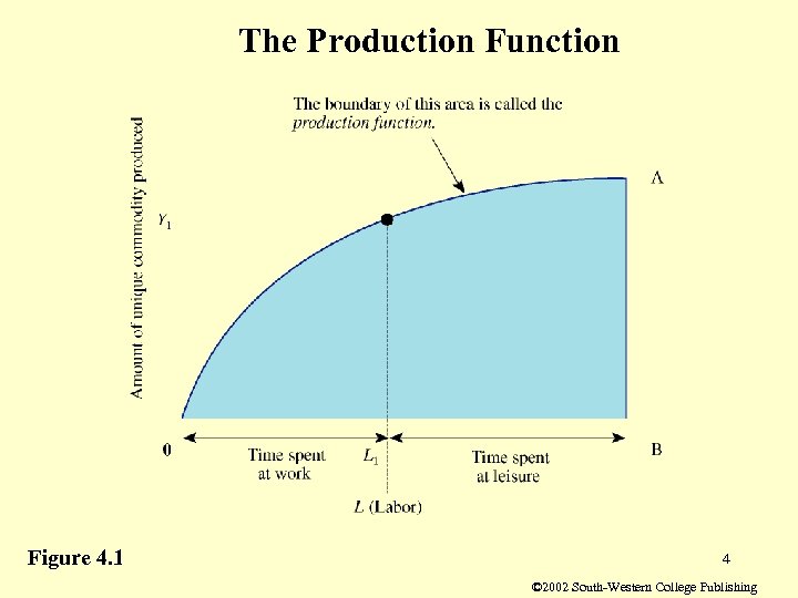The Production Function Figure 4. 1 4 © 2002 South-Western College Publishing

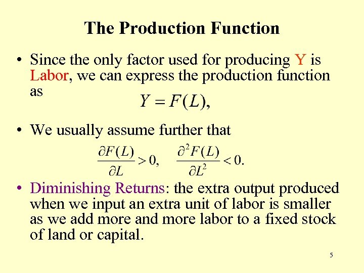The Production Function • Since the only factor used for producing Y is Labor, we can express the production function as • We usually assume further that • Diminishing Returns: the extra output produced when we input an extra unit of labor is smaller as we add more and more labor to a fixed stock of land or capital. 5

Competitive Market • Classical theory assumes that no one individual can influence price. • In our example, wage and price level. • We assume there are so many individuals, and so one can always buy the cheaper goods and work for the higher wage if there are. 6

The Nominal and Real Wage • In this chapter, we do not try to explain why money is used or how money price are set. • The nominal wage: The money paid to the worker for each hour of work. • The real wage: the amount of final commodity that a firm must give up to purchase an hour of labor time. 7

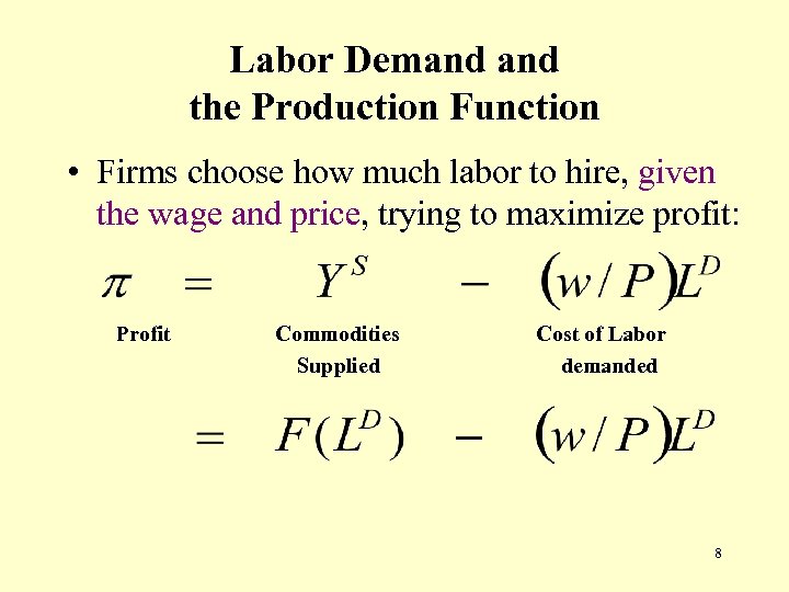Labor Demand the Production Function • Firms choose how much labor to hire, given the wage and price, trying to maximize profit: Profit Commodities Supplied Cost of Labor demanded 8

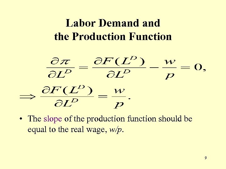Labor Demand the Production Function • The slope of the production function should be equal to the real wage, w/p. 9

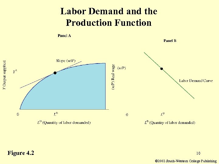Labor Demand the Production Function Figure 4. 2 10 © 2002 South-Western College Publishing

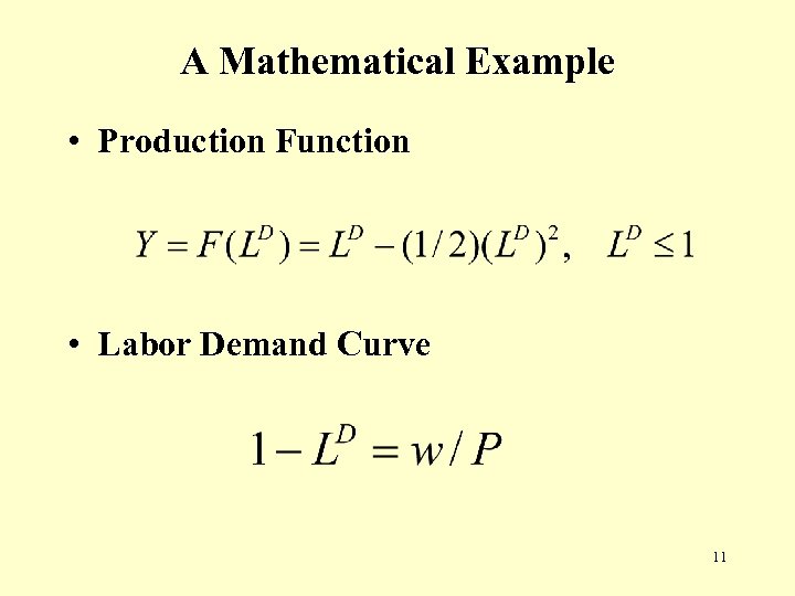A Mathematical Example • Production Function • Labor Demand Curve 11

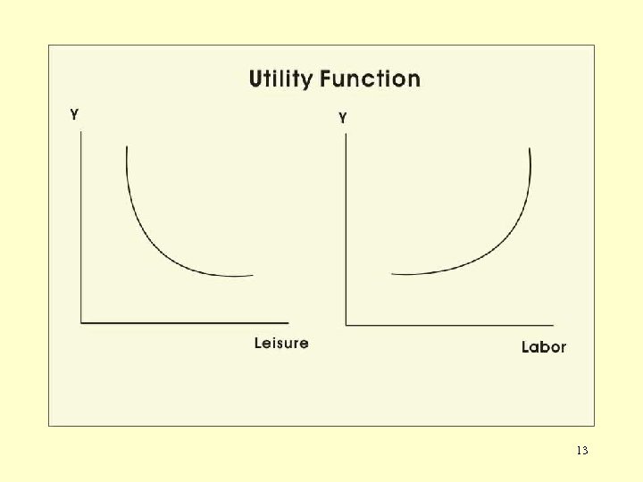
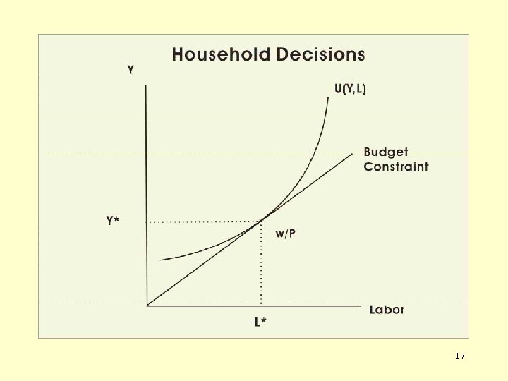
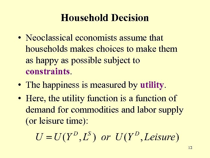Household Decision • Neoclassical economists assume that households makes choices to make them as happy as possible subject to constraints. • The happiness is measured by utility. • Here, the utility function is a function of demand for commodities and labor supply (or leisure time): 12

13

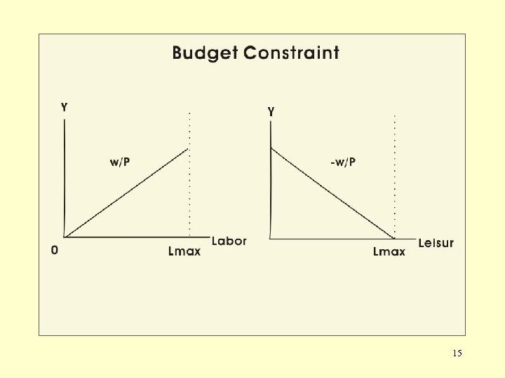
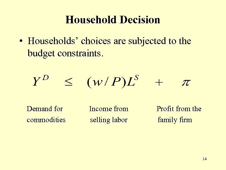Household Decision • Households’ choices are subjected to the budget constraints. Demand for commodities Income from selling labor Profit from the family firm 14

15

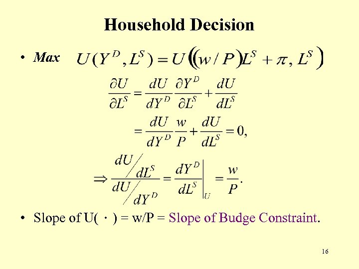Household Decision • Max • Slope of U(．) = w/P = Slope of Budge Constraint. 16

17

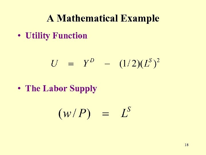A Mathematical Example • Utility Function • The Labor Supply 18

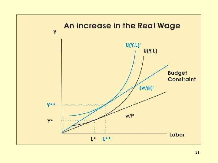
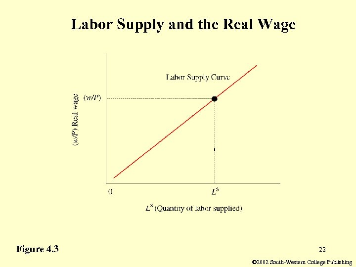
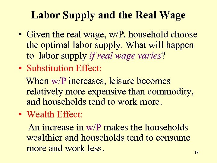Labor Supply and the Real Wage • Given the real wage, w/P, household choose the optimal labor supply. What will happen to labor supply if real wage varies? • Substitution Effect: When w/P increases, leisure becomes relatively more expensive than commodity, and households tend to work more. • Wealth Effect: An increase in w/P makes the households wealthier and households tend to consume more and work less. 19

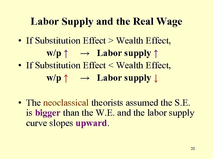Labor Supply and the Real Wage • If Substitution Effect > Wealth Effect, w/p ↑ → Labor supply ↑ • If Substitution Effect < Wealth Effect, w/p ↑ → Labor supply ↓ • The neoclassical theorists assumed the S. E. is bigger than the W. E. and the labor supply curve slopes upward. 20

21

Labor Supply and the Real Wage Figure 4. 3 22 © 2002 South-Western College Publishing

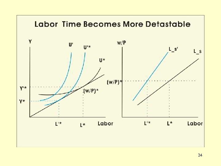
Factors that Shift Labor Supply • Preference (Utility Function): If leisure become more preferable (detestable) than labor time (or commodity (Y) ), this will lead to a shift of the labor supply. Ex. Labor time becomes more detestable. Necessary condition: Slope of U(．) = w/P Since U(Y, L) becomes steeper, labor supply will decrease given the same w/p. 23

24

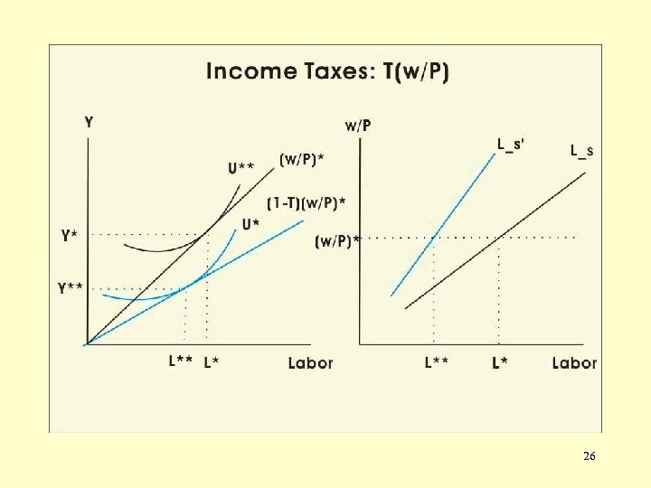
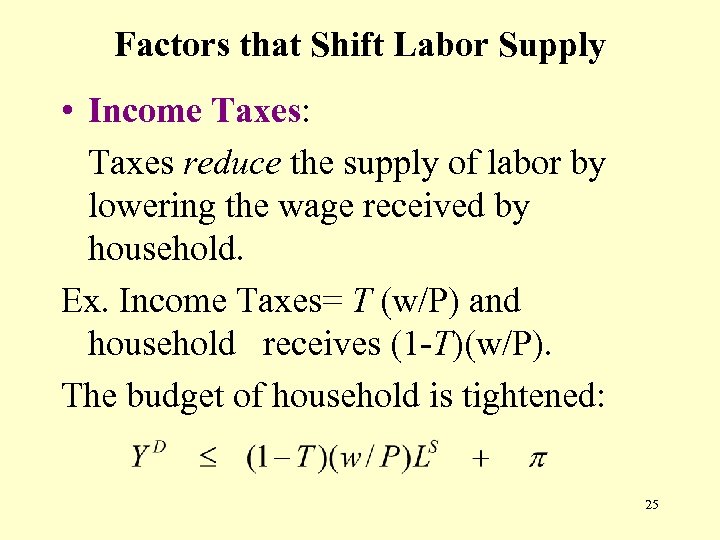Factors that Shift Labor Supply • Income Taxes: Taxes reduce the supply of labor by lowering the wage received by household. Ex. Income Taxes= T (w/P) and household receives (1 -T)(w/P). The budget of household is tightened: 25

26

27

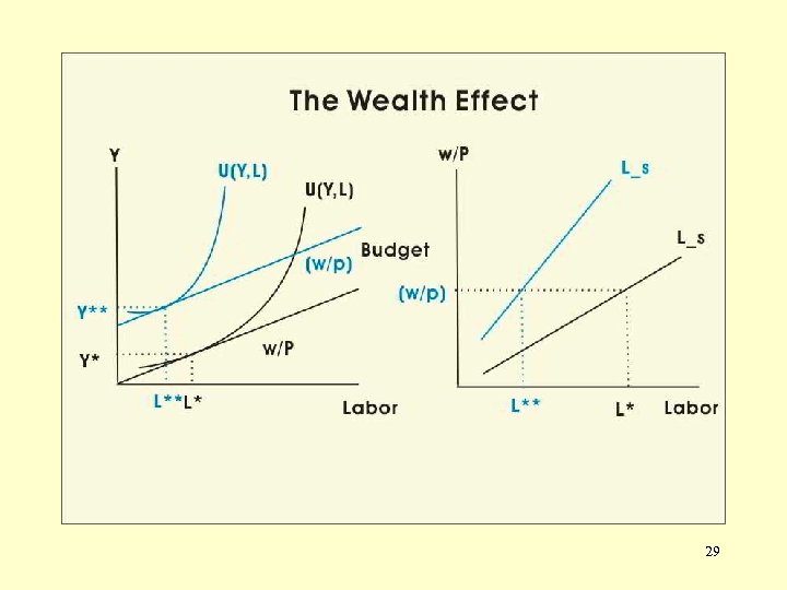
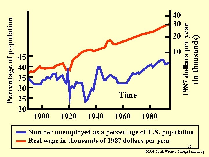
Factors that Shift Labor Supply • The Wealth Effect: As households get richer, if all other thing remain equal, they work fewer hours. Empirical: The effect of increasing wealth on labor supply is offset by the rise in the real wage. 28

29

45 40 35 30 25 20 10 Time 1900 1920 1940 1960 1987 dollars per year (in thousands) Percentage of population 40 30 20 1980 Number unemployed as a percentage of U. S. population Real wage in thousands of 1987 dollars per year 30 © 1999 South-Western College Publishing

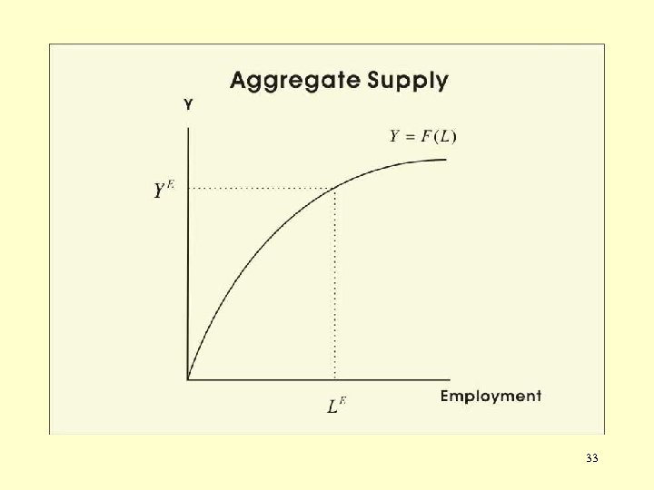
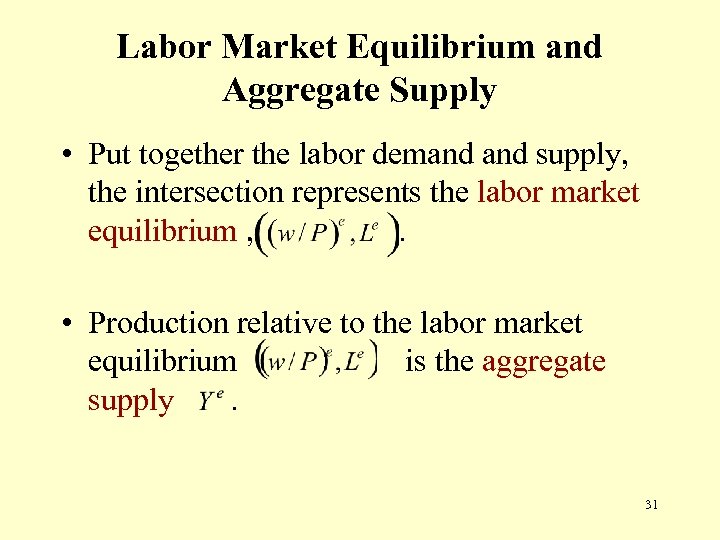Labor Market Equilibrium and Aggregate Supply • Put together the labor demand supply, the intersection represents the labor market equilibrium , . • Production relative to the labor market equilibrium is the aggregate supply. 31

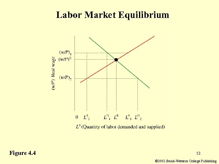Labor Market Equilibrium Figure 4. 4 32 © 2002 South-Western College Publishing

33

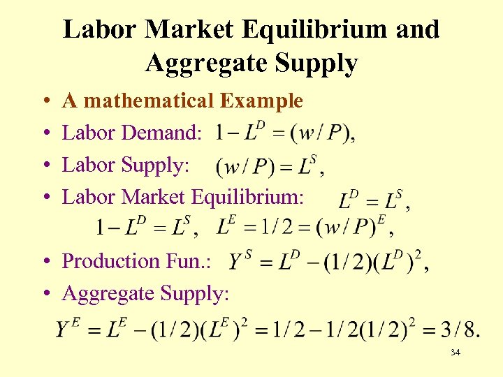Labor Market Equilibrium and Aggregate Supply • • A mathematical Example Labor Demand: Labor Supply: Labor Market Equilibrium: • Production Fun. : • Aggregate Supply: 34

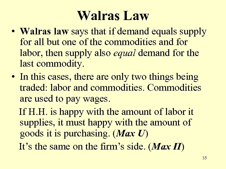Walras Law • Walras law says that if demand equals supply for all but one of the commodities and for labor, then supply also equal demand for the last commodity. • In this cases, there are only two things being traded: labor and commodities. Commodities are used to pay wages. If H. H. is happy with the amount of labor it supplies, it must happy with the amount of goods it is purchasing. (Max U) It’s the same on the firm’s side. (Max Π) 35

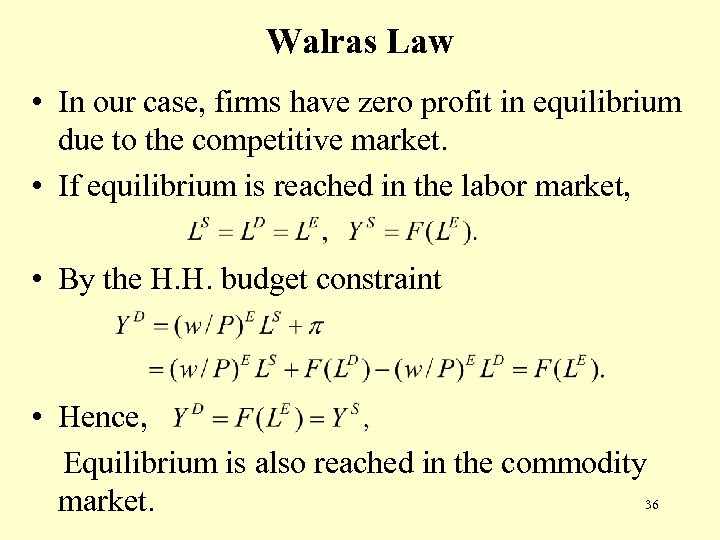Walras Law • In our case, firms have zero profit in equilibrium due to the competitive market. • If equilibrium is reached in the labor market, • By the H. H. budget constraint • Hence, Equilibrium is also reached in the commodity 36 market.

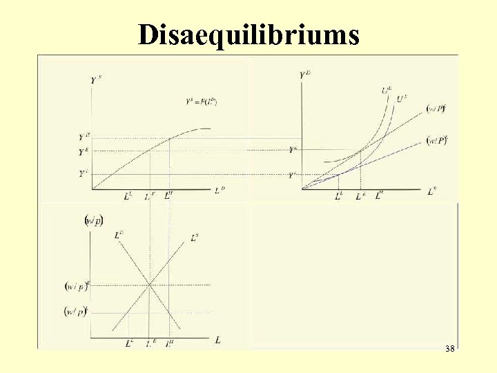
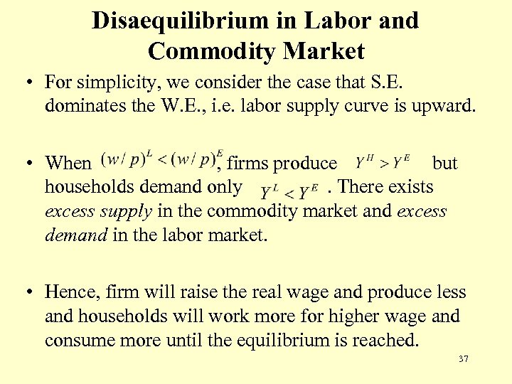Disaequilibrium in Labor and Commodity Market • For simplicity, we consider the case that S. E. dominates the W. E. , i. e. labor supply curve is upward. • When , firms produce but households demand only. There exists excess supply in the commodity market and excess demand in the labor market. • Hence, firm will raise the real wage and produce less and households will work more for higher wage and consume more until the equilibrium is reached. 37

Disaequilibriums 38

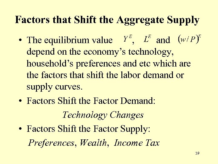Factors that Shift the Aggregate Supply • The equilibrium value , and depend on the economy’s technology, household’s preferences and etc which are the factors that shift the labor demand or supply curves. • Factors Shift the Factor Demand: Technology Changes • Factors Shift the Factor Supply: Preferences, Wealth, Income Tax 39

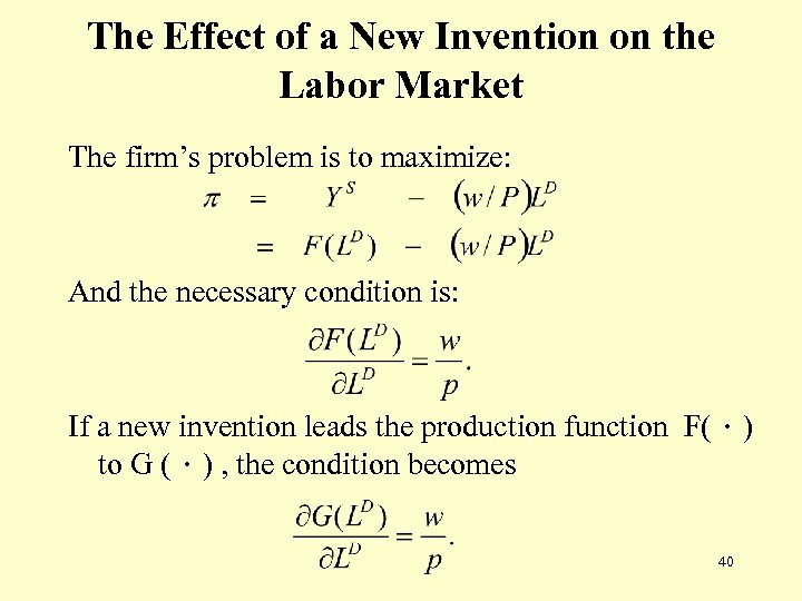The Effect of a New Invention on the Labor Market The firm’s problem is to maximize: And the necessary condition is: If a new invention leads the production function F(．) to G (．) , the condition becomes 40

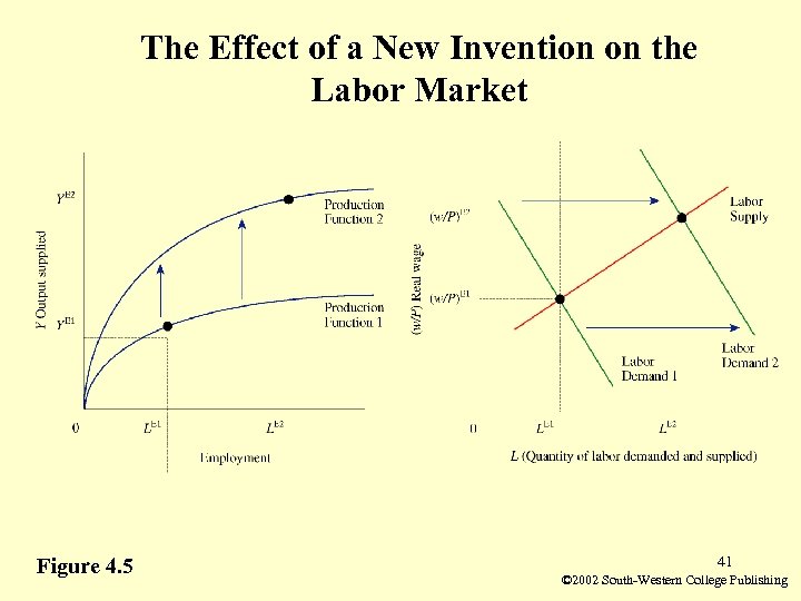The Effect of a New Invention on the Labor Market Figure 4. 5 41 © 2002 South-Western College Publishing

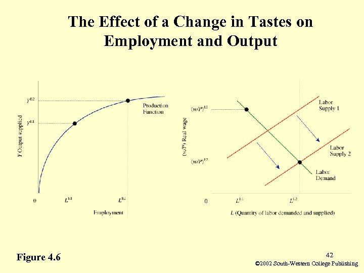The Effect of a Change in Tastes on Employment and Output Figure 4. 6 42 © 2002 South-Western College Publishing

Real Business Cycles (RBC) • The RBC economists believe that random shocks to technology account for 70% of post. World War II business cycle fluctuations. (See Figure 4. 7) and the classical revival is so called the RBC school. • In the RBC economy, fluctuations are the unavoidable responses of optimizing agents to changing productive opportunities, and there is no role for policy because the agents react in the most efficient way possible. 43

Real Business Cycles (RBC) • Many macroeconomists are hostile to the revival of the classical model: 1. The RBC model provides a partial explanation of economic fluctuations, but it is not the whole story. 2. The RBC model pays little or no attention to unemployment. • Even though, the idea that demand equals supply is now widely used by modern researchers in macroeconomics. 44

Homework Question 2, 4, 6, 8, 9 45

END