Chapter 4 Multi-Variable Control Topics Synthesis of

Chapter 4 Multi-Variable Control

Topics Synthesis of Configurations for Multiple-Input, Multiple-Output Processes ¡ Interaction Analysis and Decoupling Methods ¡ Optimal Control Approaches ¡

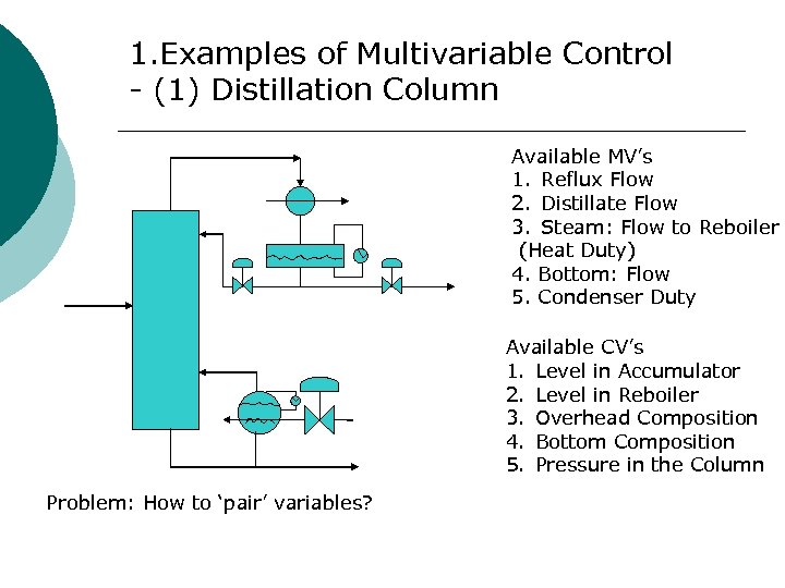
1. Examples of Multivariable Control - (1) Distillation Column Available MV’s 1. Reflux Flow 2. Distillate Flow 3. Steam: Flow to Reboiler (Heat Duty) 4. Bottom: Flow 5. Condenser Duty Available CV’s 1. Level in Accumulator 2. Level in Reboiler 3. Overhead Composition 4. Bottom Composition 5. Pressure in the Column Problem: How to ‘pair’ variables?

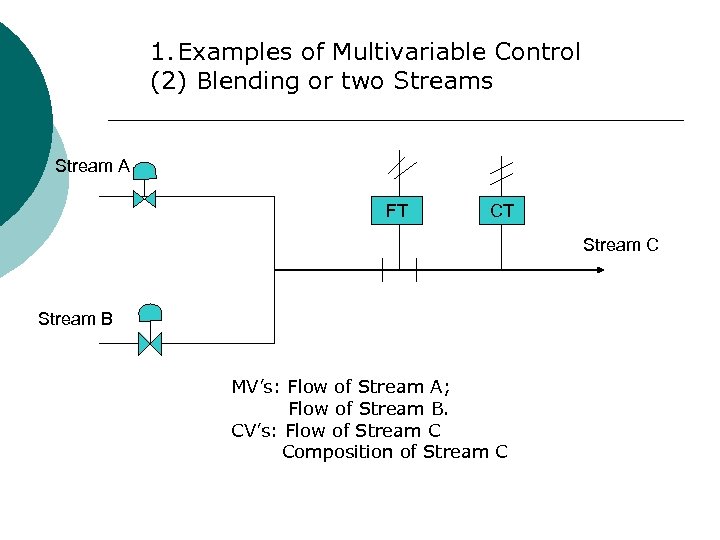
1. Examples of Multivariable Control (2) Blending or two Streams Stream A FT CT Stream C Stream B MV’s: Flow of Stream A; Flow of Stream B. CV’s: Flow of Stream C Composition of Stream C

Examples of Multivariable Control: (3) Control of a Mixing Tank Hot Cold LT TT MV’s: Flow of Hot Stream Flow of Cold Stream CV’s: Level in the tank Temperature in the tank

2. Issue of Degree of Freedom (DOF) ¡ ¡ Question: How many variables can be measured and controlled? Answer: The number of variables to be controlled is related to the degree of freedom of a system. l F=V-E ¡ ¡ If F>0, then F variables must be either (1) externally defined or (2)throught a control system To control n CV’s, we need n MV’s.

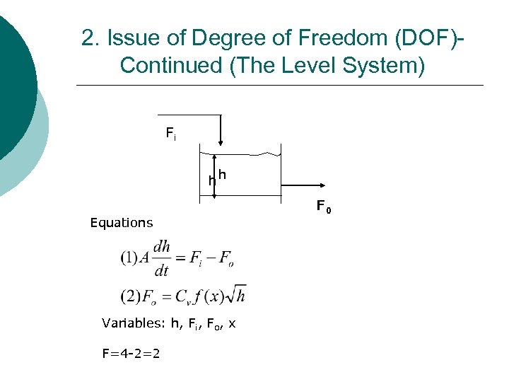
2. Issue of Degree of Freedom (DOF)Continued (The Level System) Fi hh Equations Variables: h, Fi, Fo, x F=4 -2=2 F 0

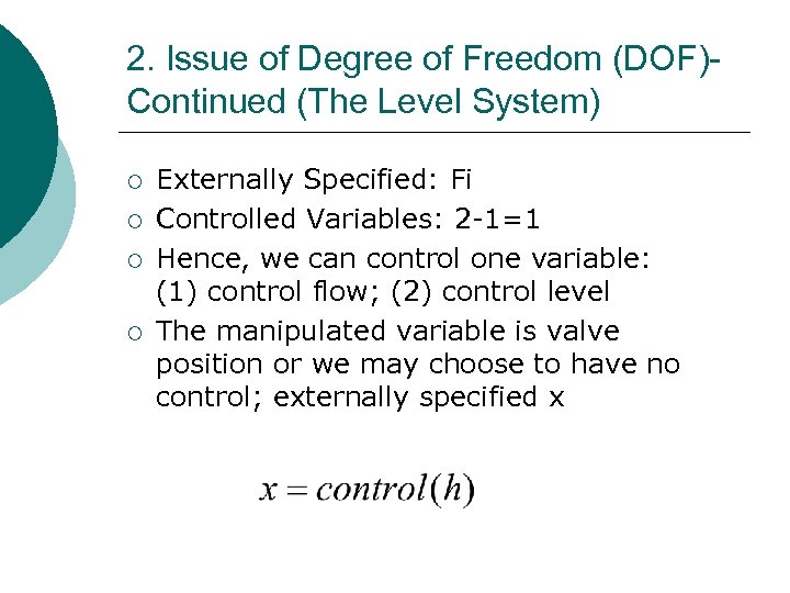
2. Issue of Degree of Freedom (DOF)Continued (The Level System) ¡ ¡ Externally Specified: Fi Controlled Variables: 2 -1=1 Hence, we can control one variable: (1) control flow; (2) control level The manipulated variable is valve position or we may choose to have no control; externally specified x

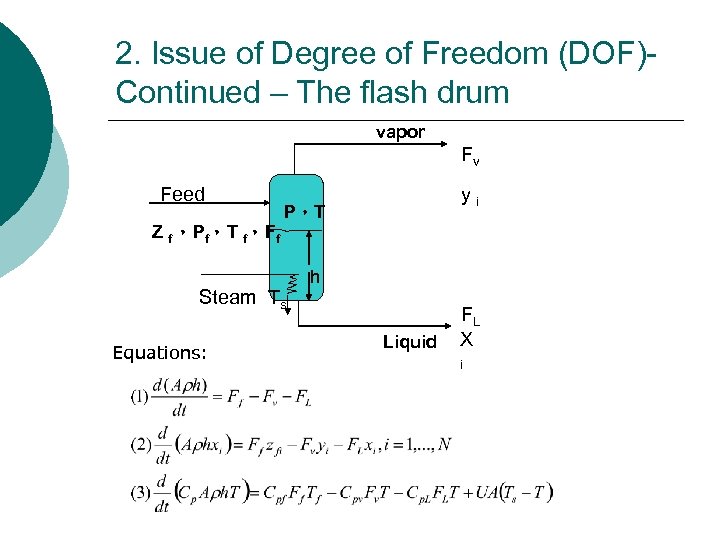
2. Issue of Degree of Freedom (DOF)Continued – The flash drum vapor Fv Feed yi P，T Z f ，Pf，T f，Ff Steam Ts Equations: h Liquid FL X i

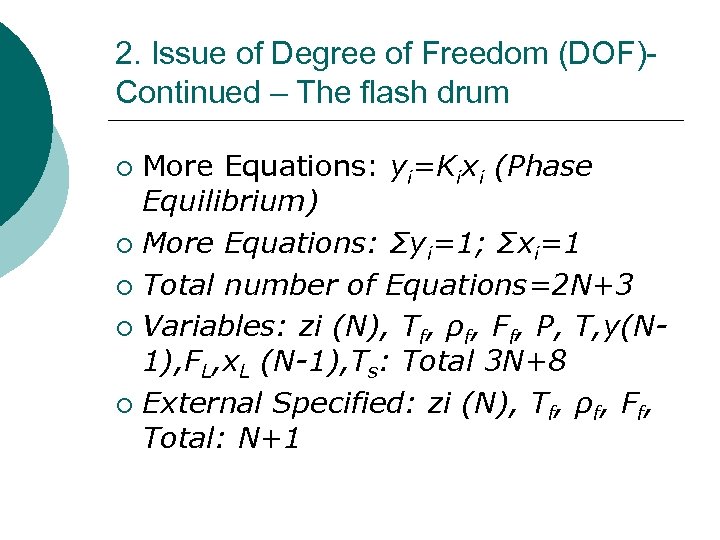
2. Issue of Degree of Freedom (DOF)Continued – The flash drum More Equations: yi=Kixi (Phase Equilibrium) ¡ More Equations: Σyi=1; Σxi=1 ¡ Total number of Equations=2 N+3 ¡ Variables: zi (N), Tf, ρf, Ff, P, T, y(N 1), FL, x. L (N-1), Ts: Total 3 N+8 ¡ External Specified: zi (N), Tf, ρf, Ff, Total: N+1 ¡

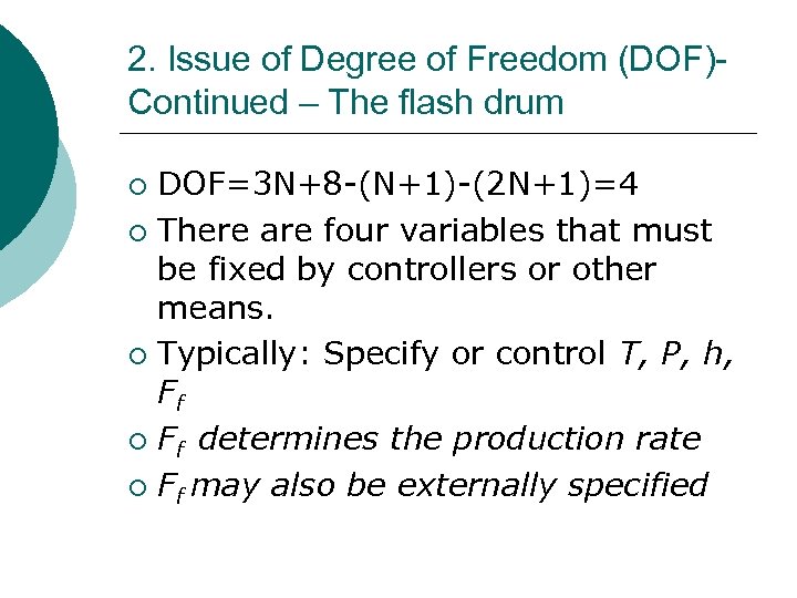
2. Issue of Degree of Freedom (DOF)Continued – The flash drum DOF=3 N+8 -(N+1)-(2 N+1)=4 ¡ There are four variables that must be fixed by controllers or other means. ¡ Typically: Specify or control T, P, h, Ff ¡ Ff determines the production rate ¡ Ff may also be externally specified ¡

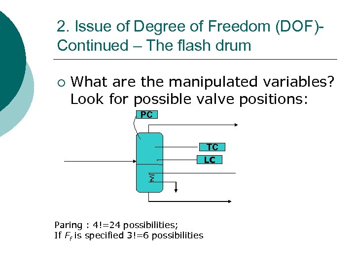
2. Issue of Degree of Freedom (DOF)Continued – The flash drum ¡ What are the manipulated variables? Look for possible valve positions: PC . Paring : 4!=24 possibilities; If Ff is specified 3!=6 possibilities TC LC

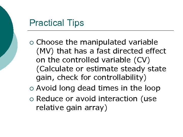
Practical Tips Choose the manipulated variable (MV) that has a fast directed effect on the controlled variable (CV) (Calculate or estimate steady state gain, check for controllability) ¡ Avoid long dead times in the loop ¡ Reduce or avoid interaction (use relative gain array) ¡

3. Interaction Problem ¡ ¡ ¡ Consider a process with two inputs and two outputs. Two control loops can be established. Question: Will actions in one loop affect the other loop? Answer: Most often, yes. This is called interaction Interaction is usually decremented to control loop performance

Approaches ¡ Design single loop controllers and detune them such that one loop does not degrade another loop performance Ø Ø ¡ Modify controlled or manipulated variables such that interaction is reduced Ø Ø ¡ ¡ not always possible selection of pairing very important Steady state interaction Dynamic interaction Determine interacting element’s transfer functions and try to compensate for them Solve the multivariable control problem (such as model predictive control –MPC)

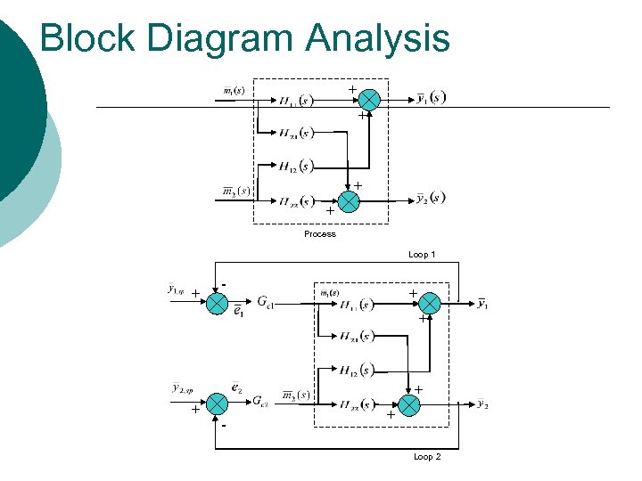
Block Diagram Analysis + + Process Loop 1 + - + Loop 2

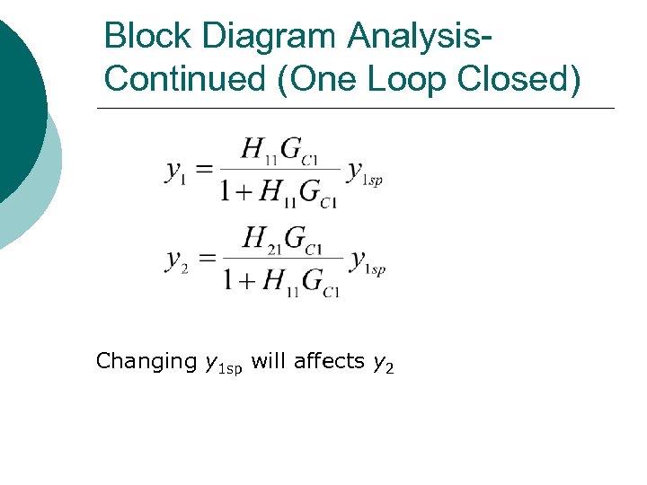
Block Diagram Analysis. Continued (One Loop Closed) Changing y 1 sp will affects y 2

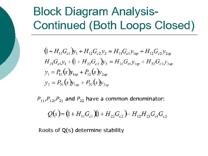
Block Diagram Analysis. Continued (Both Loops Closed) P 11, P 12, P 21 and P 22 have a common denominator: Roots of Q(s) determine stability

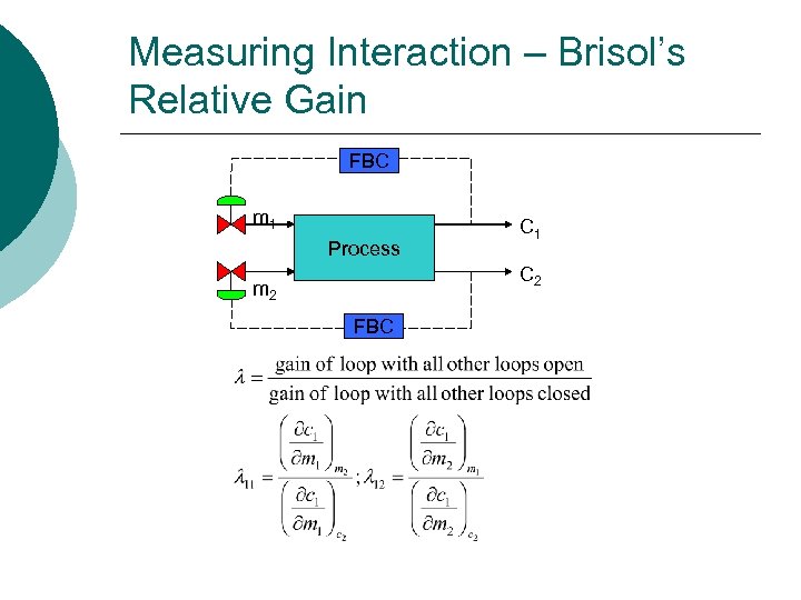
Measuring Interaction – Brisol’s Relative Gain FBC m 1 Process C 1 C 2 m 2 FBC

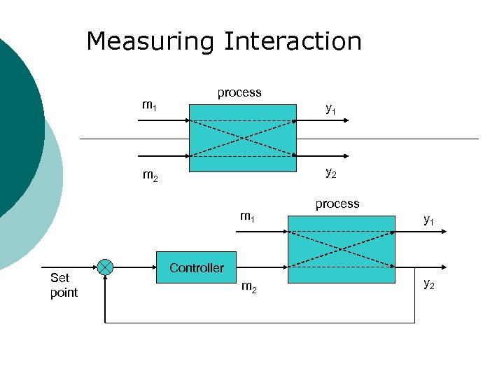
Measuring Interaction m 1 process y 1 y 2 m 1 Set point Controller m 2 process y 1 y 2

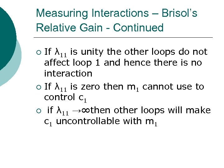
Measuring Interactions – Brisol’s Relative Gain - Continued If λ 11 is unity the other loops do not affect loop 1 and hence there is no interaction ¡ If λ 11 is zero then m 1 cannot use to control c 1 ¡ if λ 11 →∞then other loops will make c 1 uncontrollable with m 1 ¡

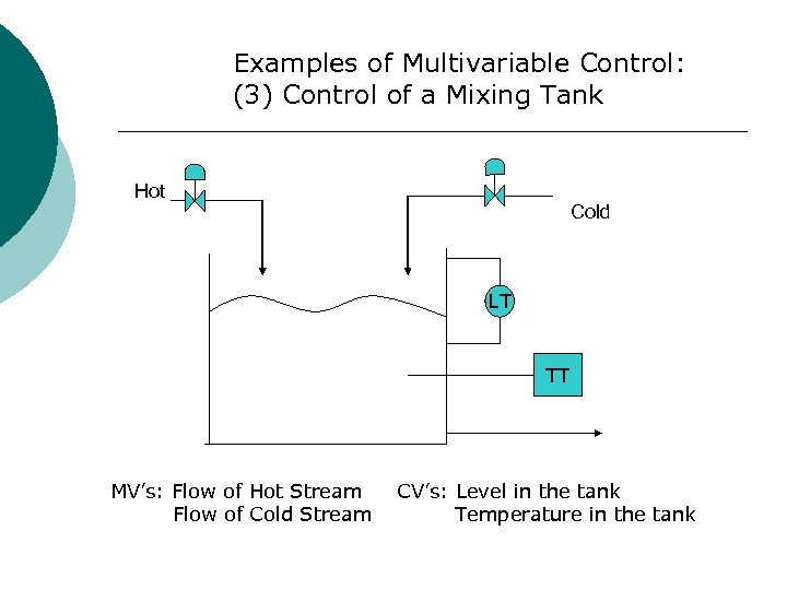
Examples of Multivariable Control: (3) Control of a Mixing Tank Hot Cold LT TT MV’s: Flow of Hot Stream Flow of Cold Stream CV’s: Level in the tank Temperature in the tank

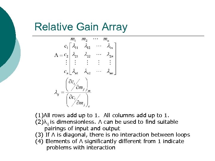
Relative Gain Array (1)All rows add up to 1. All columns add up to 1. (2)λij is dimensionless. Λ can be used to find suitable pairings of input and output (3) If Λ is diagonal, there is no interaction between loops (4) Elements of Λ significantly different from 1 indicate problems with interaction

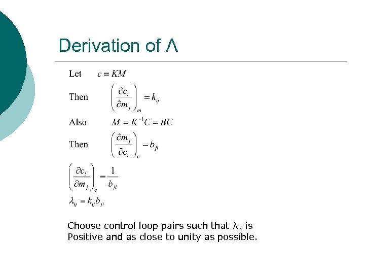
Derivation of Λ Choose control loop pairs such that λij is Positive and as close to unity as possible.

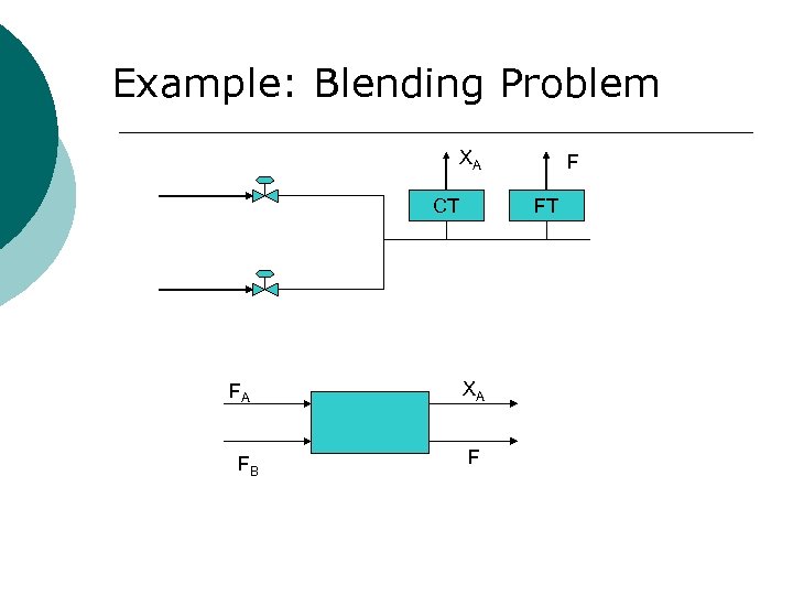
Example: Blending Problem XA CT FA FB F FT XA F

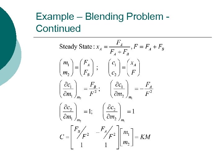
Example – Blending Problem Continued

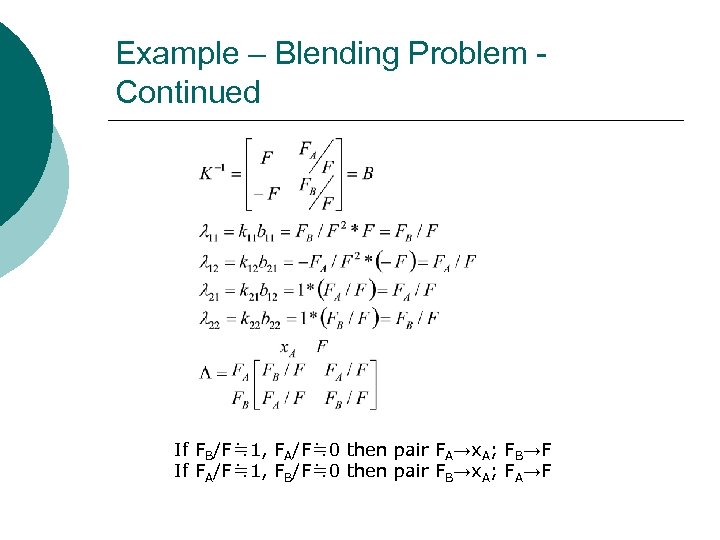
Example – Blending Problem Continued If FB/F≒ 1, FA/F≒ 0 then pair FA→x. A; FB→F If FA/F≒ 1, FB/F≒ 0 then pair FB→x. A; FA→F

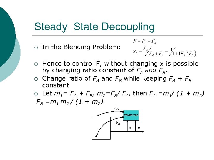
Steady State Decoupling ¡ In the Blending Problem: Hence to control F, without changing x is possible by changing ratio constant of FA and FB. ¡ Change ratio of FA and FB while keeping FA + FB constant ¡ Let m 1= FA + FB, m 2=FB/ FA, then FA =m 1/ (1 + m 2) FB =m 1 m 2 / (1 + m 2) ¡ FA COMPUTER FB F X

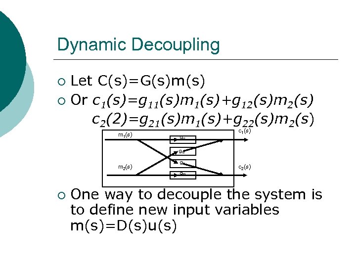
Dynamic Decoupling Let C(s)=G(s)m(s) ¡ Or c 1(s)=g 11(s)m 1(s)+g 12(s)m 2(s) c 2(2)=g 21(s)m 1(s)+g 22(s)m 2(s) ¡ m 1(s) g 11 c 1(s) g 12 m 2(s) ¡ g 21 g 22 c 2(s) One way to decouple the system is to define new input variables m(s)=D(s)u(s)

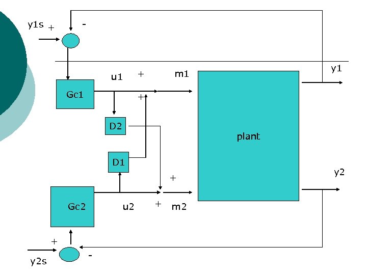
Dynamic Decoupling-Continued If D(s) is a matrix, then c(s)=G(s)D(s)u(s) ¡ If D(s) is chosen such that G(s)D(s)=diagonal, then ¡ u 1(s) affects only c 1, u 2 only affects c 2. ¡ The system is called decoupled. ¡

y 1 s + - u 1 Gc 1 + + D 2 plant D 1 + Gc 2 u 2 + y 2 s y 1 m 1 - + m 2 y 2

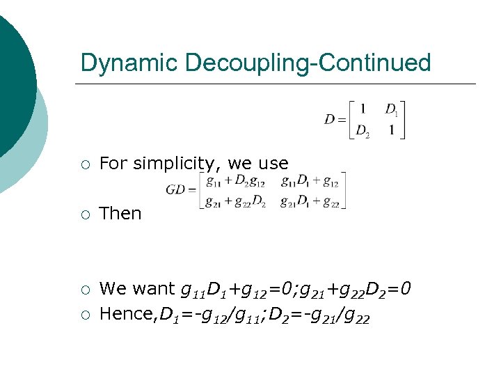
Dynamic Decoupling-Continued ¡ For simplicity, we use ¡ Then ¡ We want g 11 D 1+g 12=0; g 21+g 22 D 2=0 Hence, D 1=-g 12/g 11; D 2=-g 21/g 22 ¡

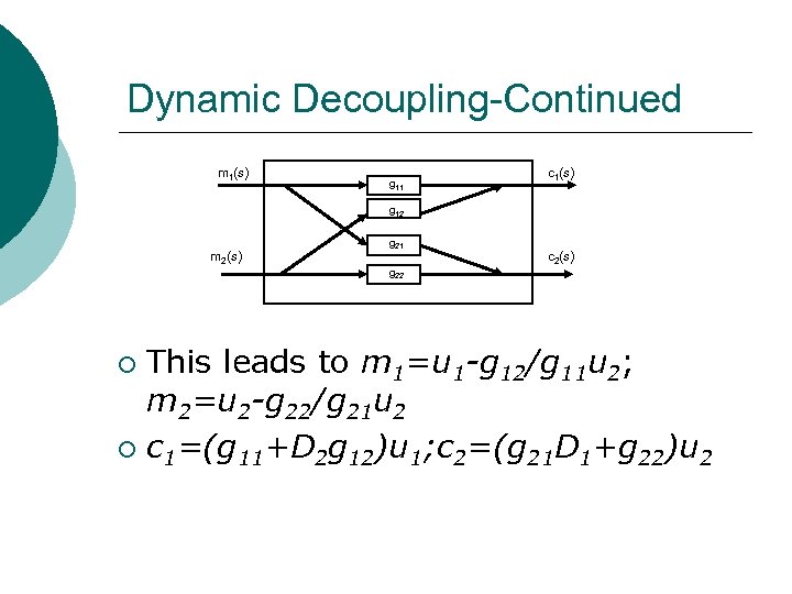
Dynamic Decoupling-Continued m 1(s) g 11 c 1(s) g 12 m 2(s) g 21 g 22 c 2(s) This leads to m 1=u 1 -g 12/g 11 u 2; m 2=u 2 -g 22/g 21 u 2 ¡ c 1=(g 11+D 2 g 12)u 1; c 2=(g 21 D 1+g 22)u 2 ¡

Conclusion Multivariable control is essential in the industrial applications ¡ Steady state decoupling is very useful in case of no dynamic system such as mixing ¡ Dynamic decoupling is very important for high valued-added system such as distillation systems ¡

Homework #4 Multivariable Systems Textbook p 698 ¡ 21. 3, 21. 4, 21. 7, 21. 8 ¡