1f17d00e9ebe431bd1ddeb5a6ab4db7a.ppt
- Количество слайдов: 77
CHAPTER 4 INVENTORY MANAGEMENT
LEARNING OBJECTIVES l Define inventory l Conduct an ABC analysis. inventory and functions l Explain of and apply the EOQ and POQ model to solve typical problems. l Compute a ROP and safety stock
Inventory l. A stock or store of goods l A stock of item kept to meet demand l Inventory Management ¡ How much ¡ When ¡ Classified ¡ Accuracy
Objective of Inventory Control l To achieve satisfactory levels of customer service while keeping inventory costs within reasonable bounds l To keep enough inventory to meet customer demand also be cost effective. ¡ Level of customer service ¡ Costs of ordering and carrying inventory
Functions of Inventory l To meet anticipated demand l To decouple operations l To protect against stock-outs l To take advantage of order cycles l To help hedge against price increases l To take advantage of quantity discounts
Types of Inventory
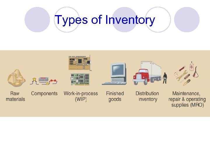
Types of Inventory l Raw material ¡ Purchased but not processed l Work-in-process ¡ Undergone some change but not completed ¡ A function of cycle time for a product l Maintenance/repair/operating (MRO) ¡ Necessary to keep machinery and processes productive
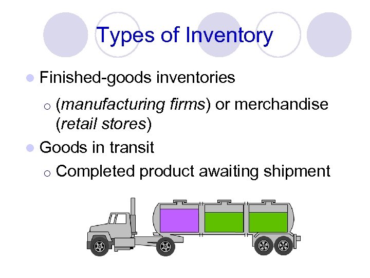
Types of Inventory l Finished-goods inventories (manufacturing firms) or merchandise (retail stores) l Goods in transit ¡ Completed product awaiting shipment ¡
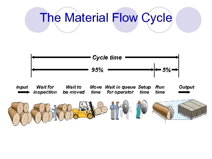
The Material Flow Cycle time 95% Input Wait for inspection Wait to be moved 5% Move Wait in queue Setup Run time for operator time Output
Effective Inventory Management l A system to keep track of inventory l A reliable forecast of demand l Knowledge of lead times l Reasonable estimates of o o Ordering costs o l Holding costs Shortage costs A classification system
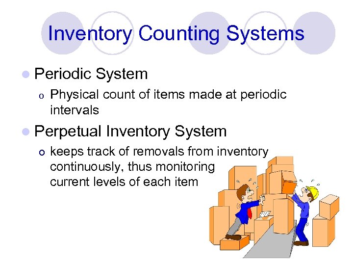
Inventory Counting Systems l Periodic o System Physical count of items made at periodic intervals l Perpetual Inventory System o keeps track of removals from inventory continuously, thus monitoring current levels of each item
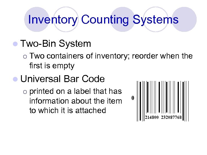
Inventory Counting Systems l Two-Bin ¡ System Two containers of inventory; reorder when the first is empty l Universal ¡ Bar Code printed on a label that has information about the item to which it is attached 0 214800 232087768
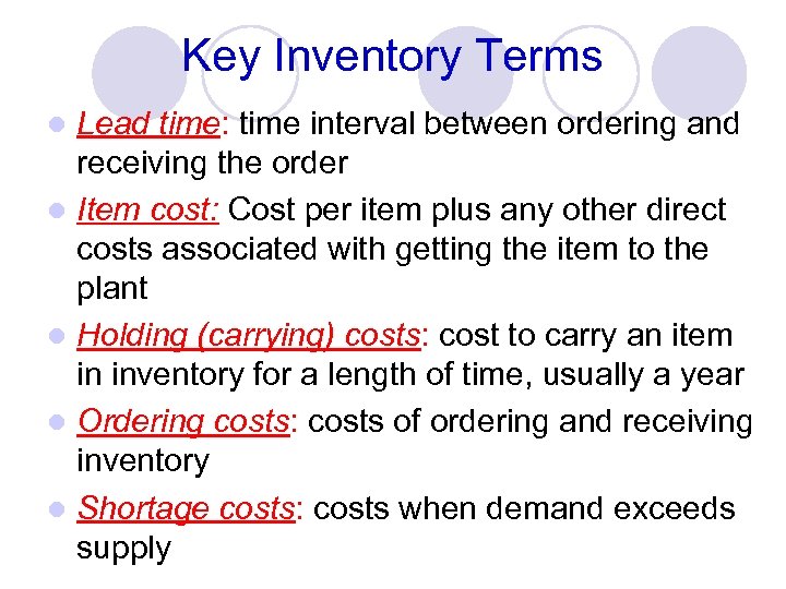
Key Inventory Terms Lead time: time interval between ordering and receiving the order l Item cost: Cost per item plus any other direct costs associated with getting the item to the plant l Holding (carrying) costs: cost to carry an item in inventory for a length of time, usually a year l Ordering costs: costs of ordering and receiving inventory l Shortage costs: costs when demand exceeds supply l
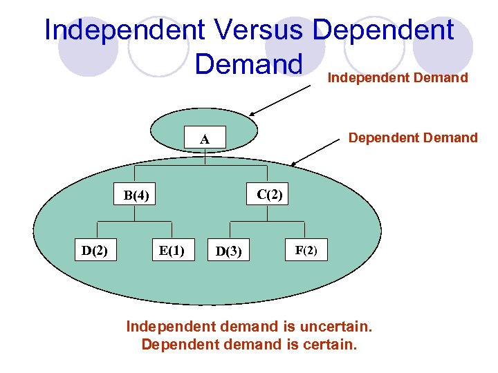
Independent Versus Dependent Demand Independent Demand Dependent Demand A C(2) B(4) D(2) E(1) D(3) F(2) Independent demand is uncertain. Dependent demand is certain.
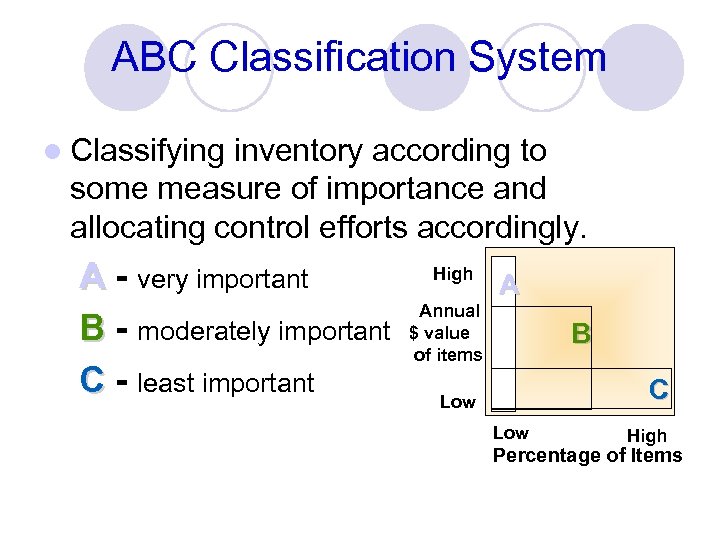
ABC Classification System l Classifying inventory according to some measure of importance and allocating control efforts accordingly. A - very important B - moderately important C - least important High A Annual $ value of items B C Low High Percentage of Items
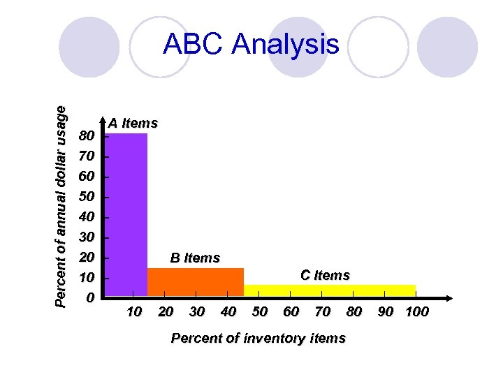
Percent of annual dollar usage ABC Analysis 80 70 60 50 40 30 20 10 0 A Items – – – – B Items – | | – 10 20 30 40 C Items | | 50 60 70 80 Percent of inventory items | | 90 100
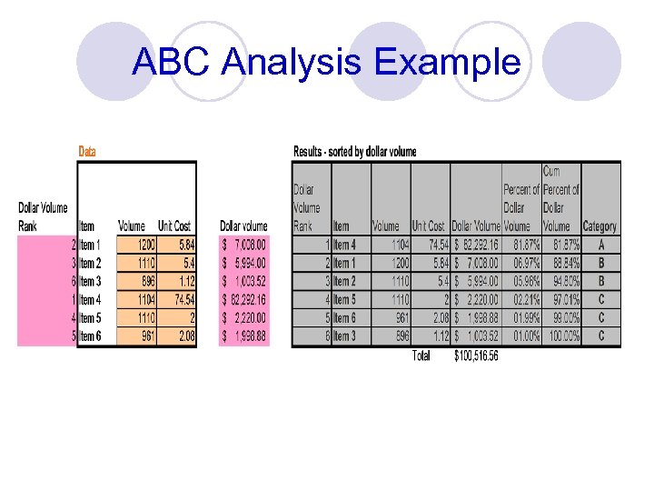
ABC Analysis Example
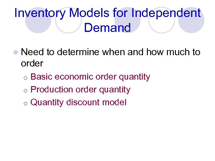
Inventory Models for Independent Demand l Need to determine when and how much to order Basic economic order quantity ¡ Production order quantity ¡ Quantity discount model ¡
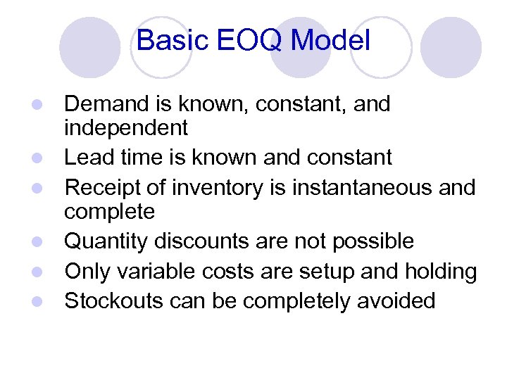
Basic EOQ Model l l l Demand is known, constant, and independent Lead time is known and constant Receipt of inventory is instantaneous and complete Quantity discounts are not possible Only variable costs are setup and holding Stockouts can be completely avoided
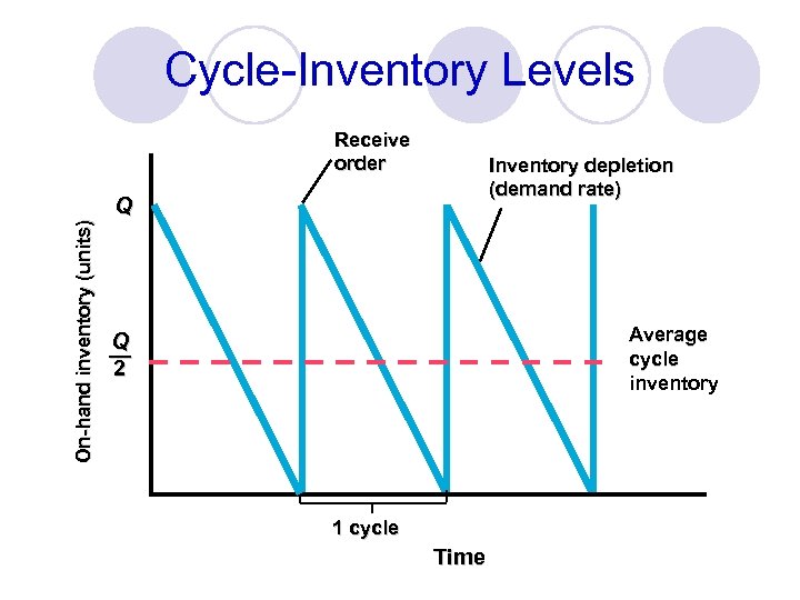
Cycle-Inventory Levels On-hand inventory (units) Receive order Inventory depletion (demand rate) Q Average cycle inventory Q — 2 1 cycle Time
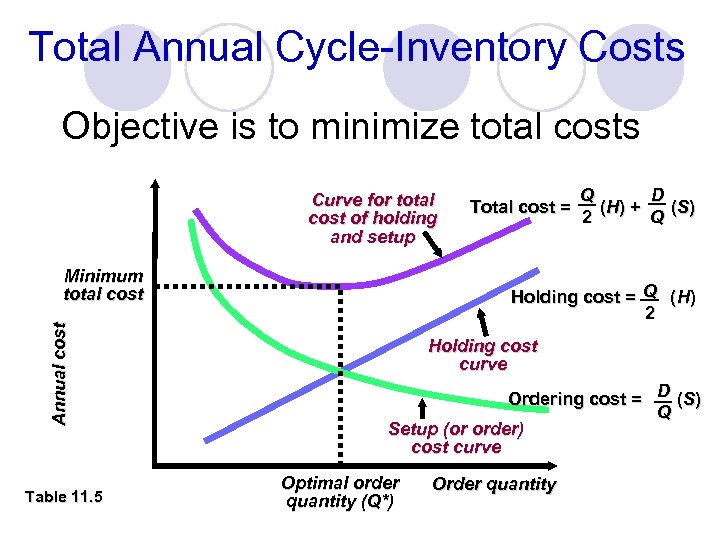
Total Annual Cycle-Inventory Costs Objective is to minimize total costs Curve for total cost of holding and setup Annual cost Minimum total cost Table 11. 5 Q D Total cost = ( H) + ( S) 2 Q Holding cost = Q (H) 2 Holding cost curve Ordering cost = D (S) Q Setup (or order) cost curve Optimal order quantity (Q*) Order quantity
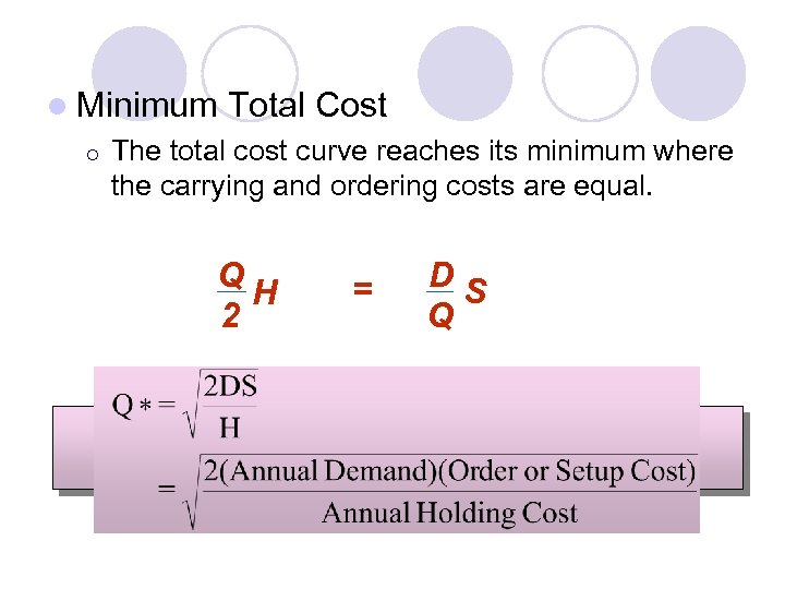
l Minimum ¡ Total Cost The total cost curve reaches its minimum where the carrying and ordering costs are equal. Q H 2 = DS Q
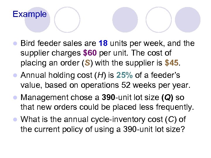
Example Bird feeder sales are 18 units per week, and the supplier charges $60 per unit. The cost of placing an order (S) with the supplier is $45. l Annual holding cost (H) is 25% of a feeder’s value, based on operations 52 weeks per year. l Management chose a 390 -unit lot size (Q) so that new orders could be placed less frequently. l What is the annual cycle-inventory cost (C) of the current policy of using a 390 -unit lot size? l
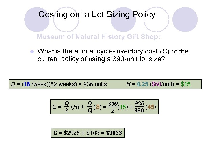
Costing out a Lot Sizing Policy Museum of Natural History Gift Shop: l What is the annual cycle-inventory cost (C) of the current policy of using a 390 -unit lot size? D = (18 /week)(52 weeks) = 936 units C= H = 0. 25 ($60/unit) = $15 Q D 936 390 (H) + (S) = (15) + (45) 2 Q 390 2 C = $2925 + $108 = $3033
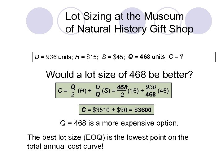
Lot Sizing at the Museum of Natural History Gift Shop Q = 468 units; D = 936 units; H = $15; S = $45; Q = 390 units; C = ? $3033 Would a lot size of 468 be better? C= Q D 936 468 (H) + (S) = (15) + (45) 2 Q 468 2 C = $3510 + $90 = $3600 Q = 468 is a more expensive option. The best lot size (EOQ) is the lowest point on the total annual cost curve!
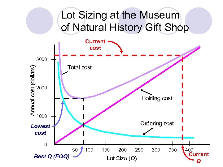
Lot Sizing at the Museum of Natural History Gift Shop Current cost Annual cost (dollars) 3000 — Total cost 2000 — Holding cost 1000 — Ordering cost Lowest cost 0 — Best Q (EOQ) | 50 | 100 | 150 | 200 | 250 Lot Size (Q) | 300 | 350 | 400 Current Q
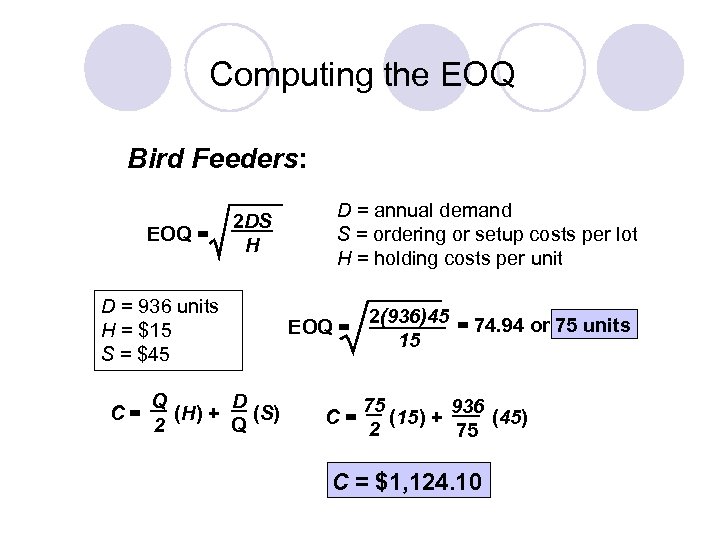
Computing the EOQ Bird Feeders: EOQ = 2 DS H D = 936 units H = $15 S = $45 C= Q D (H) + (S) 2 Q D = annual demand S = ordering or setup costs per lot H = holding costs per unit EOQ = C= 2(936)45 = 74. 94 or 75 units 15 75 936 (15) + (45) 2 75 C = $1, 124. 10
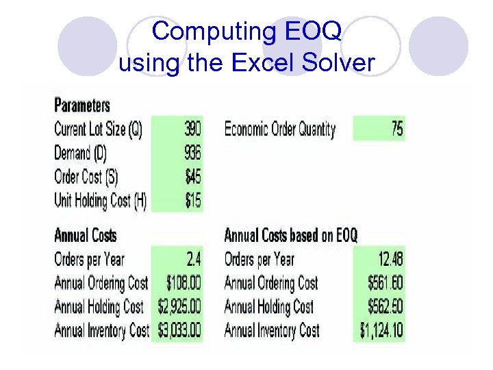
Computing EOQ using the Excel Solver
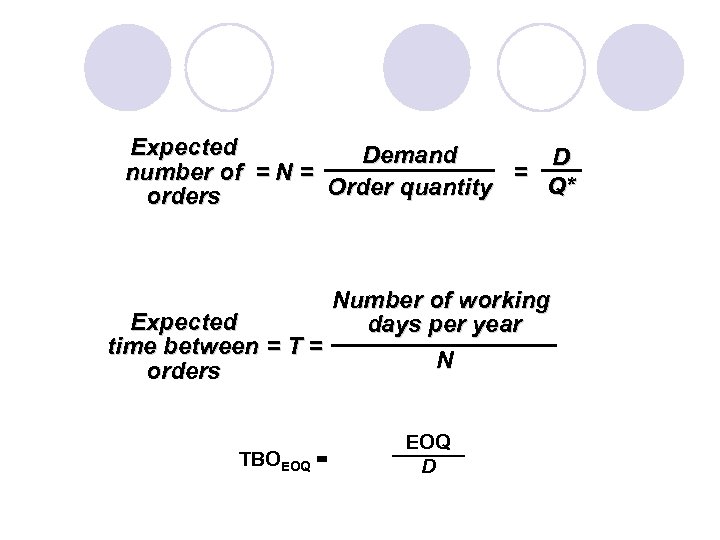
Expected Demand D number of = N = = Q* Order quantity orders Number of working Expected days per year time between = T = N orders TBOEOQ = EOQ D
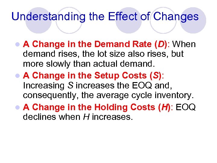
Understanding the Effect of Changes A Change in the Demand Rate (D): When demand rises, the lot size also rises, but more slowly than actual demand. l A Change in the Setup Costs (S): Increasing S increases the EOQ and, consequently, the average cycle inventory. l A Change in the Holding Costs (H): EOQ declines when H increases. l
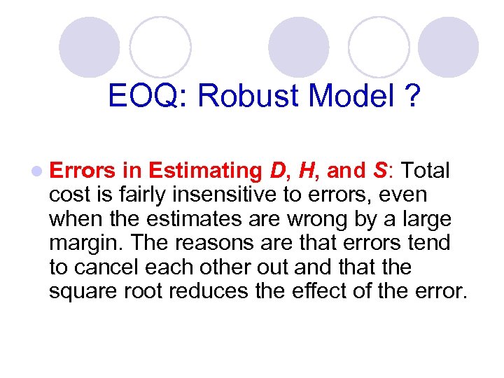
EOQ: Robust Model ? l Errors in Estimating D, H, and S: Total cost is fairly insensitive to errors, even when the estimates are wrong by a large margin. The reasons are that errors tend to cancel each other out and that the square root reduces the effect of the error.
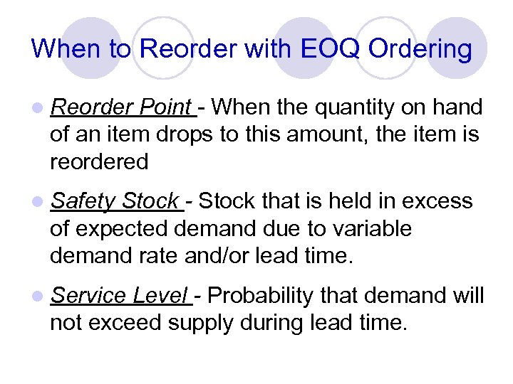
When to Reorder with EOQ Ordering l Reorder Point - When the quantity on hand of an item drops to this amount, the item is reordered l Safety Stock - Stock that is held in excess of expected demand due to variable demand rate and/or lead time. l Service Level - Probability that demand will not exceed supply during lead time.
Determinants of the Reorder Point l The rate of demand l The lead time l Demand and/or lead time variability l Stockout risk (safety stock)
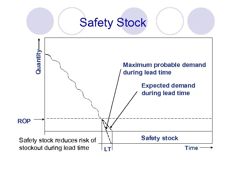
Quantity Safety Stock Maximum probable demand during lead time Expected demand during lead time ROP Safety stock reduces risk of stockout during lead time Safety stock LT Time
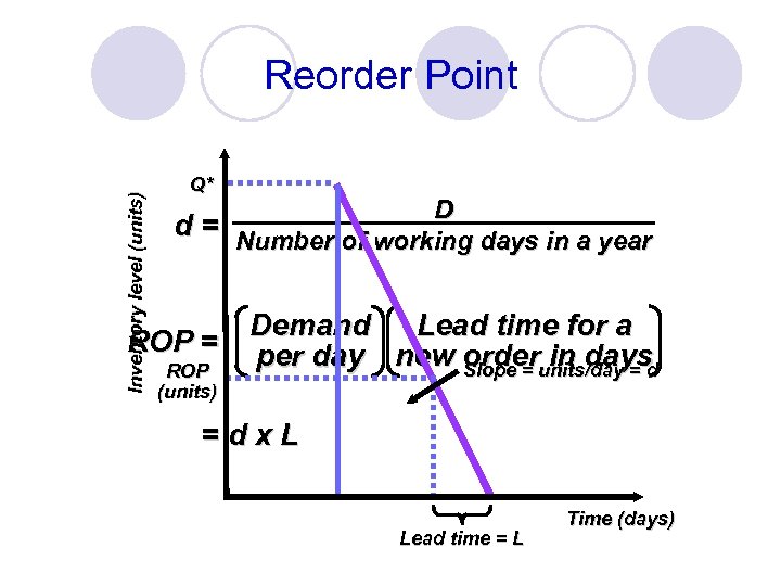
Inventory level (units) Reorder Point Q* D d = Number of working days in a year Lead time for a Demand ROP = per day new order in days Slope = units/day = d ROP (units) =dx. L Lead time = L Time (days)
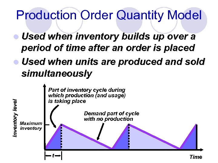
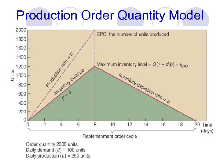
Production Order Quantity Model l Used when inventory builds up over a Inventory level period of time after an order is placed l Used when units are produced and sold simultaneously Part of inventory cycle during which production (and usage) is taking place Demand part of cycle with no production Maximum inventory t Time
Production Order Quantity Model
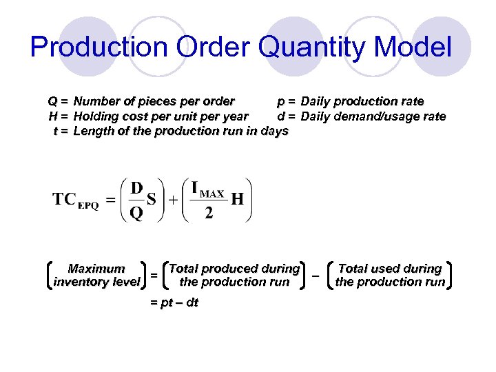
Production Order Quantity Model Q = Number of pieces per order p = Daily production rate H = Holding cost per unit per year d = Daily demand/usage rate t = Length of the production run in days Total produced during Maximum = – the production run inventory level = pt – dt Total used during the production run
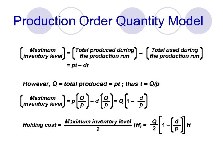
Production Order Quantity Model Total produced during Maximum = – the production run inventory level Total used during the production run = pt – dt However, Q = total produced = pt ; thus t = Q/p Q Maximum =p inventory level p Holding cost = –d Q p =Q 1– d p Maximum inventory level Q d (H ) = 1– 2 p 2 H
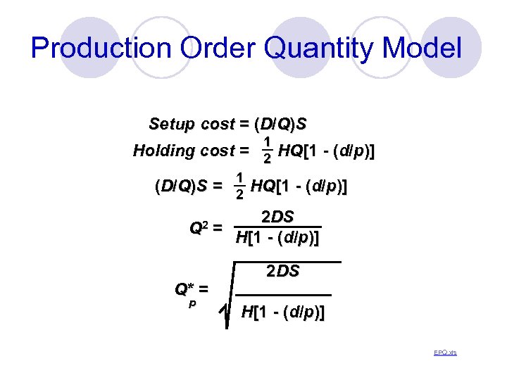
Production Order Quantity Model Setup cost = (D/Q)S 1 Holding cost = 2 HQ[1 - (d/p)] (D / Q )S = Q 2 Q* = p 1 2 HQ[1 - (d/p)] 2 DS = H[1 - (d/p)] 2 DS H[1 - (d/p)] EPQ. xls
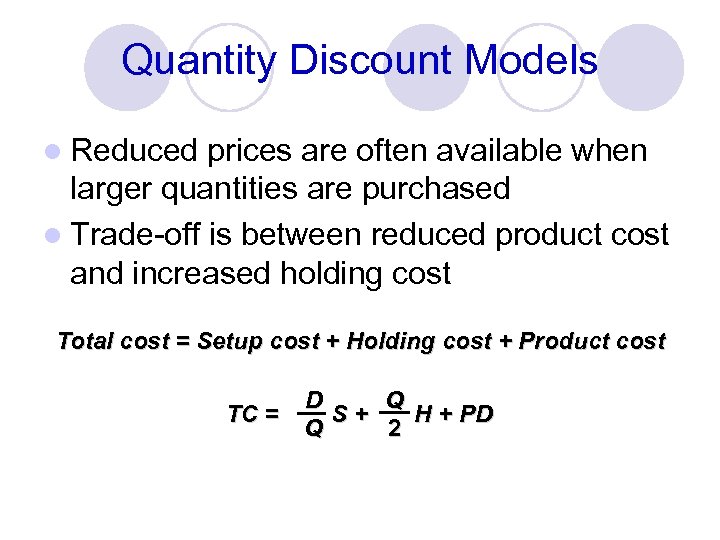
Quantity Discount Models l Reduced prices are often available when larger quantities are purchased l Trade-off is between reduced product cost and increased holding cost Total cost = Setup cost + Holding cost + Product cost TC = D Q S+ H + PD Q 2
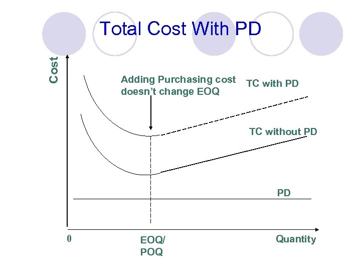
Cost Total Cost With PD Adding Purchasing cost doesn’t change EOQ TC with PD TC without PD PD 0 EOQ/ POQ Quantity
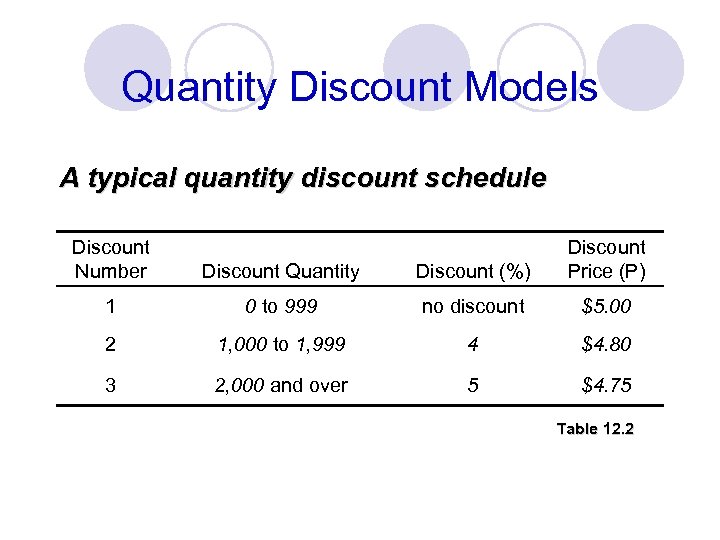
Quantity Discount Models A typical quantity discount schedule Discount Number Discount Quantity Discount (%) Discount Price (P) 1 0 to 999 no discount $5. 00 2 1, 000 to 1, 999 4 $4. 80 3 2, 000 and over 5 $4. 75 Table 12. 2
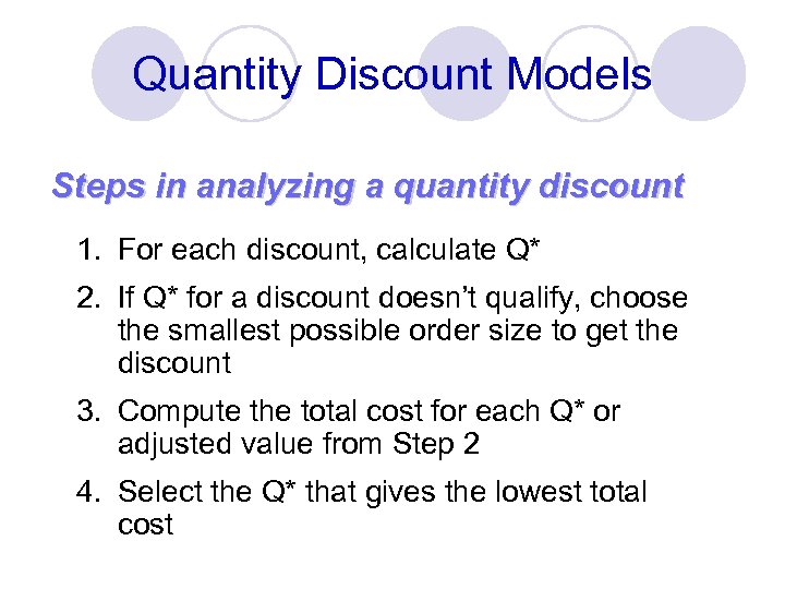
Quantity Discount Models Steps in analyzing a quantity discount 1. For each discount, calculate Q* 2. If Q* for a discount doesn’t qualify, choose the smallest possible order size to get the discount 3. Compute the total cost for each Q* or adjusted value from Step 2 4. Select the Q* that gives the lowest total cost
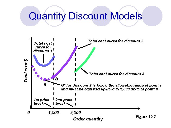
Quantity Discount Models Total cost curve for discount 2 Total cost $ Total cost curve for discount 1 b a Q* for discount 2 is below the allowable range at point a and must be adjusted upward to 1, 000 units at point b 1 st price break 0 Total cost curve for discount 3 2 nd price break 1, 000 2, 000 Order quantity Figure 12. 7
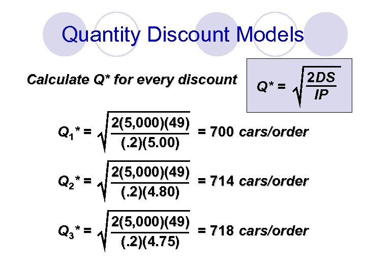
Quantity Discount Models Calculate Q* for every discount Q* = 2 DS IP Q 1* = 2(5, 000)(49) = 700 cars/order (. 2)(5. 00) Q 2* = 2(5, 000)(49) = 714 cars/order (. 2)(4. 80) Q 3* = 2(5, 000)(49) = 718 cars/order (. 2)(4. 75)
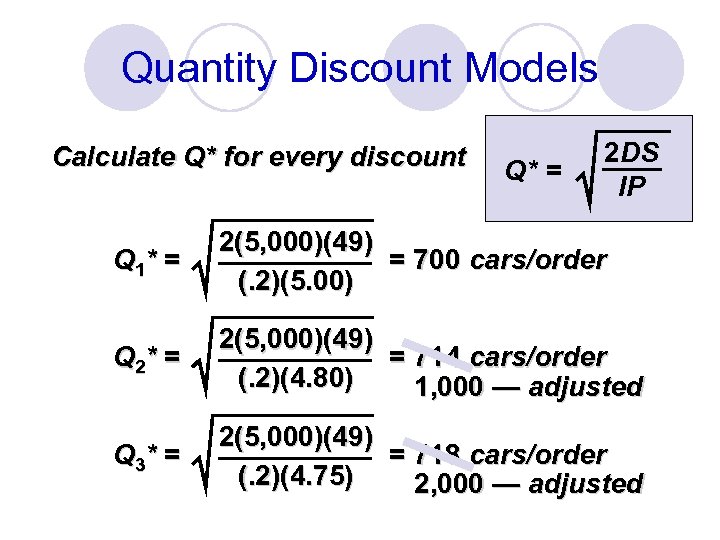
Quantity Discount Models Calculate Q* for every discount Q* = 2 DS IP Q 1* = 2(5, 000)(49) = 700 cars/order (. 2)(5. 00) Q 2* = 2(5, 000)(49) = 714 cars/order (. 2)(4. 80) 1, 000 — adjusted Q 3* = 2(5, 000)(49) = 718 cars/order (. 2)(4. 75) 2, 000 — adjusted
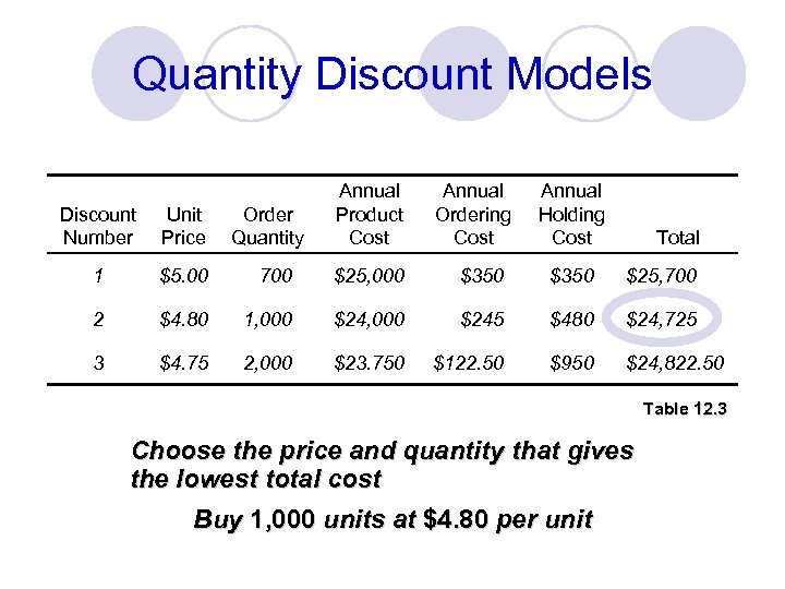
Quantity Discount Models Order Quantity Annual Product Cost Annual Ordering Cost Annual Holding Cost Discount Number Unit Price 1 $5. 00 700 $25, 000 $350 $25, 700 2 $4. 80 1, 000 $245 $480 $24, 725 3 $4. 75 2, 000 $23. 750 $122. 50 $950 $24, 822. 50 Total Table 12. 3 Choose the price and quantity that gives the lowest total cost Buy 1, 000 units at $4. 80 per unit
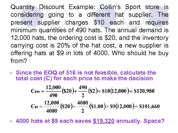
Quantity Discount Example: Collin’s Sport store is considering going to a different hat supplier. The present supplier charges $10 each and requires minimum quantities of 490 hats. The annual demand is 12, 000 hats, the ordering cost is $20, and the inventory carrying cost is 20% of the hat cost, a new supplier is offering hats at $9 in lots of 4000. Who should he buy from? l Since the EOQ of 516 is not feasible, calculate the total cost (C) for each price to make the decision l 4000 hats at $9 each saves $19, 320 annually. Space?
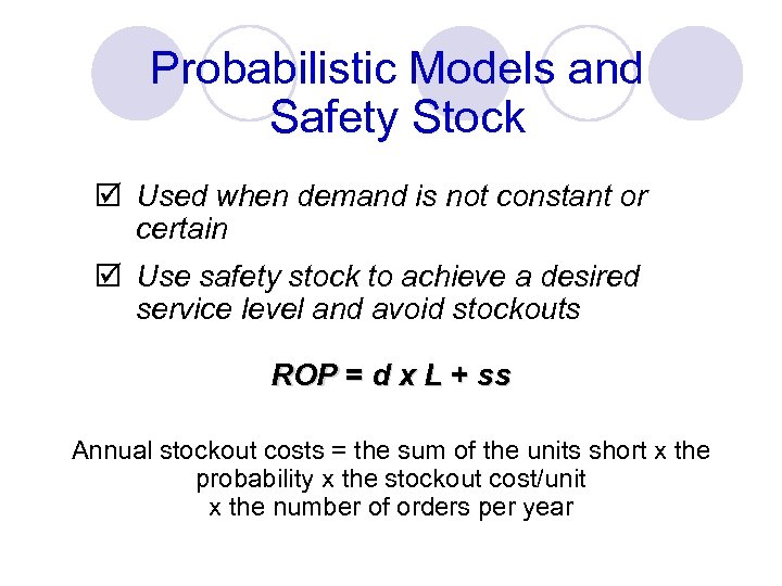
Probabilistic Models and Safety Stock þ Used when demand is not constant or certain þ Use safety stock to achieve a desired service level and avoid stockouts ROP = d x L + ss Annual stockout costs = the sum of the units short x the probability x the stockout cost/unit x the number of orders per year
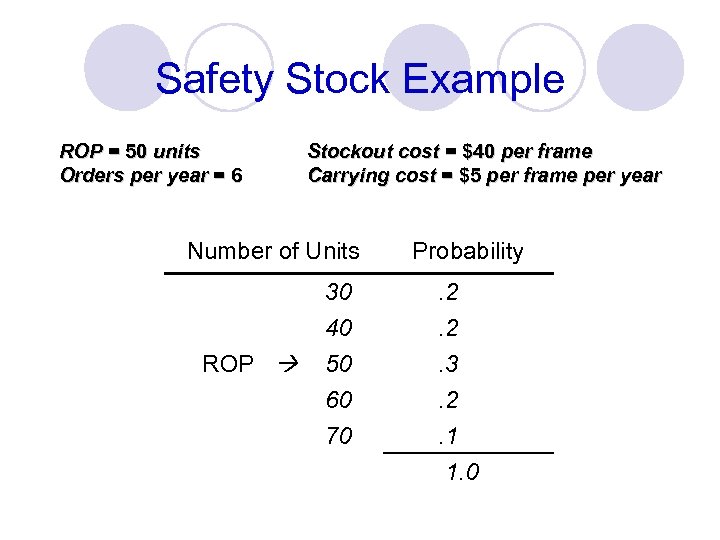
Safety Stock Example ROP = 50 units Orders per year = 6 Stockout cost = $40 per frame Carrying cost = $5 per frame per year Number of Units ROP Probability 30 40 50 . 2. 2. 3 60 70 . 2. 1 1. 0
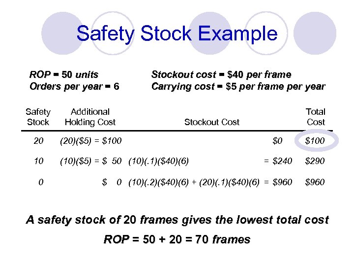
Safety Stock Example ROP = 50 units Orders per year = 6 Stockout cost = $40 per frame Carrying cost = $5 per frame per year Safety Stock Additional Holding Cost 20 (20)($5) = $100 10 (10)($5) = $ 50 (10)(. 1)($40)(6) 0 $ Total Cost Stockout Cost $0 $100 = $240 $290 0 (10)(. 2)($40)(6) + (20)(. 1)($40)(6) = $960 A safety stock of 20 frames gives the lowest total cost ROP = 50 + 20 = 70 frames
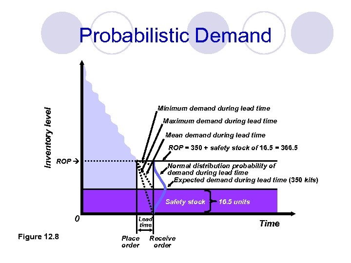
Inventory level Probabilistic Demand Minimum demand during lead time Maximum demand during lead time Mean demand during lead time ROP = 350 + safety stock of 16. 5 = 366. 5 ROP Normal distribution probability of demand during lead time Expected demand during lead time (350 kits) Safety stock 0 Figure 12. 8 Lead time Place order Receive order 16. 5 units Time
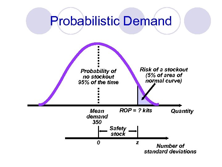
Probabilistic Demand Risk of a stockout (5% of area of normal curve) Probability of no stockout 95% of the time Mean demand 350 0 ROP = ? kits Quantity Safety stock z Number of standard deviations
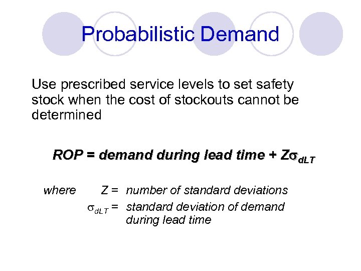
Probabilistic Demand Use prescribed service levels to set safety stock when the cost of stockouts cannot be determined ROP = demand during lead time + Z d. LT where Z = number of standard deviations sd. LT = standard deviation of demand during lead time
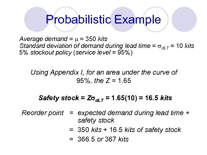
Probabilistic Example Average demand = m = 350 kits Standard deviation of demand during lead time = sd. LT = 10 kits 5% stockout policy (service level = 95%) Using Appendix I, for an area under the curve of 95%, the Z = 1. 65 Safety stock = Z d. LT = 1. 65(10) = 16. 5 kits Reorder point = expected demand during lead time + safety stock = 350 kits + 16. 5 kits of safety stock = 366. 5 or 367 kits
Other Probabilistic Models When data on demand during lead time is not available, there are other models available 1. When demand is variable and lead time is constant 2. When lead time is variable and demand is constant 3. When both demand lead time are variable
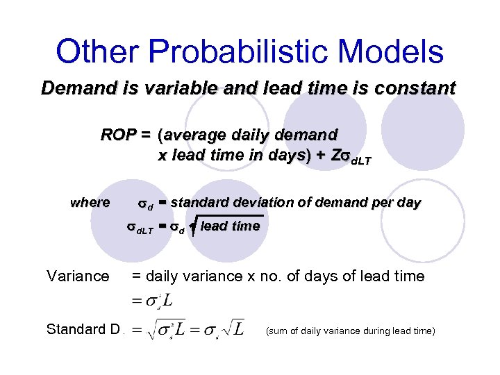
Other Probabilistic Models Demand is variable and lead time is constant ROP = (average daily demand x lead time in days) + Z d. LT where d = standard deviation of demand per day d. LT = d Variance Standard D. lead time = daily variance x no. of days of lead time (sum of daily variance during lead time)
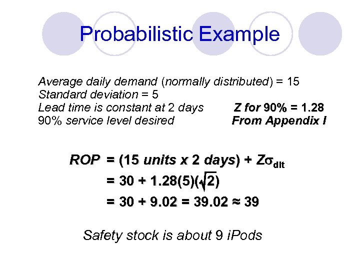
Probabilistic Example Average daily demand (normally distributed) = 15 Standard deviation = 5 Z for 90% = 1. 28 Lead time is constant at 2 days From Appendix I 90% service level desired ROP = (15 units x 2 days) + Z dlt = 30 + 1. 28(5)( 2) = 30 + 9. 02 = 39. 02 ≈ 39 Safety stock is about 9 i. Pods
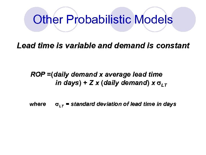
Other Probabilistic Models Lead time is variable and demand is constant ROP =(daily demand x average lead time in days) + Z x (daily demand) x LT where LT = standard deviation of lead time in days
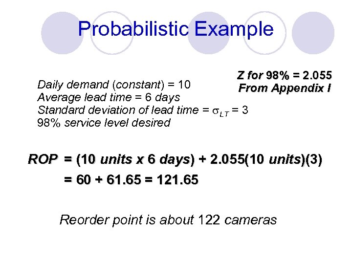
Probabilistic Example Z for 98% = 2. 055 From Appendix I Daily demand (constant) = 10 Average lead time = 6 days Standard deviation of lead time = s. LT = 3 98% service level desired ROP = (10 units x 6 days) + 2. 055(10 units)(3) = 60 + 61. 65 = 121. 65 Reorder point is about 122 cameras
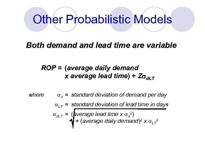
Other Probabilistic Models Both demand lead time are variable ROP = (average daily demand x average lead time) + Z d. LT where sd = standard deviation of demand per day s. LT = standard deviation of lead time in days sd. LT = (average lead time x sd 2) + (average daily demand)2 x s. LT 2
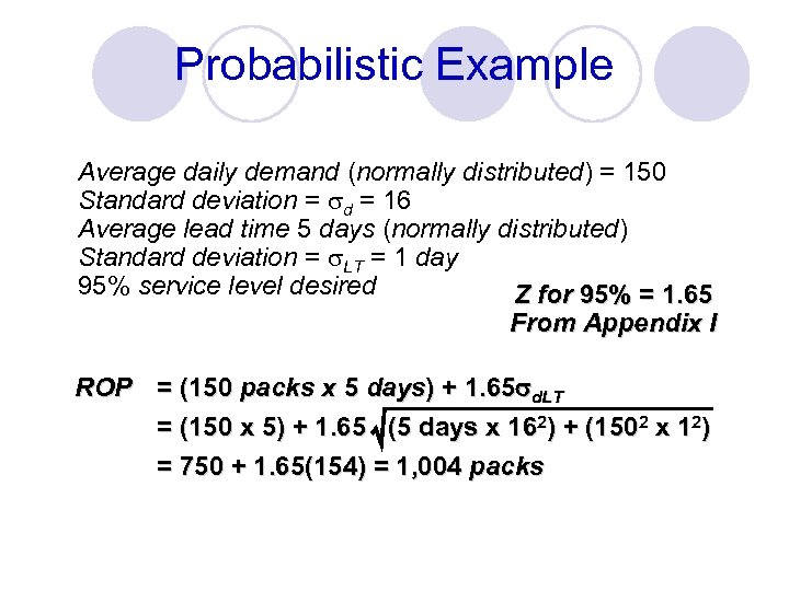
Probabilistic Example Average daily demand (normally distributed) = 150 Standard deviation = sd = 16 Average lead time 5 days (normally distributed) Standard deviation = s. LT = 1 day 95% service level desired Z for 95% = 1. 65 From Appendix I ROP = (150 packs x 5 days) + 1. 65 d. LT = (150 x 5) + 1. 65 (5 days x 162) + (1502 x 12) = 750 + 1. 65(154) = 1, 004 packs
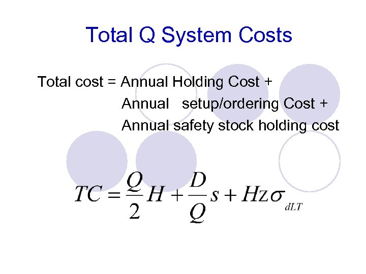
Total Q System Costs Total cost = Annual Holding Cost + Annual setup/ordering Cost + Annual safety stock holding cost
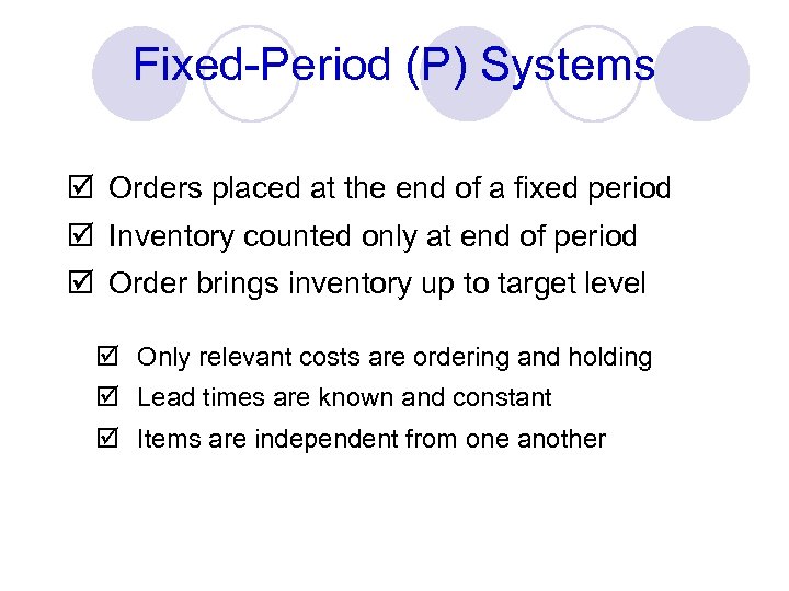
Fixed-Period (P) Systems þ Orders placed at the end of a fixed period þ Inventory counted only at end of period þ Order brings inventory up to target level þ Only relevant costs are ordering and holding þ Lead times are known and constant þ Items are independent from one another
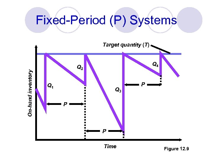
Fixed-Period (P) Systems On-hand inventory Target quantity (T) Q 4 Q 2 Q 1 Q 3 P P P Time Figure 12. 9
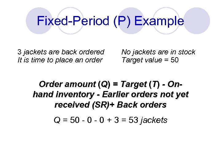
Fixed-Period (P) Example 3 jackets are back ordered It is time to place an order No jackets are in stock Target value = 50 Order amount (Q) = Target (T) - Onhand inventory - Earlier orders not yet received (SR)+ Back orders Q = 50 - 0 + 3 = 53 jackets
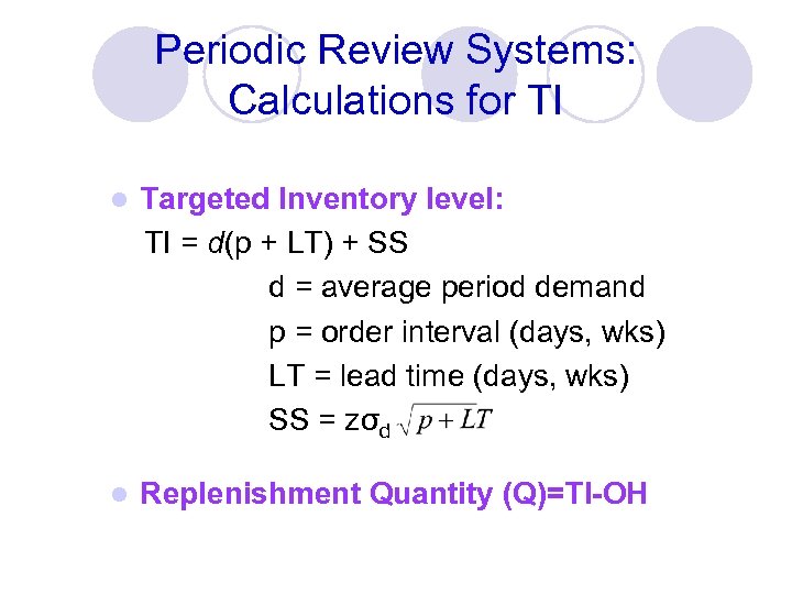
Periodic Review Systems: Calculations for TI l Targeted Inventory level: TI = d(p + LT) + SS d = average period demand p = order interval (days, wks) LT = lead time (days, wks) SS = zσd l Replenishment Quantity (Q)=TI-OH
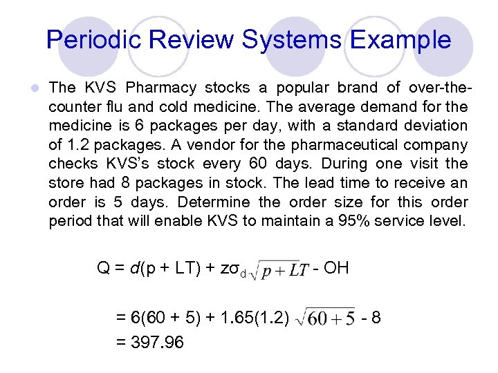
Periodic Review Systems Example l The KVS Pharmacy stocks a popular brand of over-thecounter flu and cold medicine. The average demand for the medicine is 6 packages per day, with a standard deviation of 1. 2 packages. A vendor for the pharmaceutical company checks KVS’s stock every 60 days. During one visit the store had 8 packages in stock. The lead time to receive an order is 5 days. Determine the order size for this order period that will enable KVS to maintain a 95% service level. Q = d(p + LT) + zσd = 6(60 + 5) + 1. 65(1. 2) = 397. 96 - OH -8
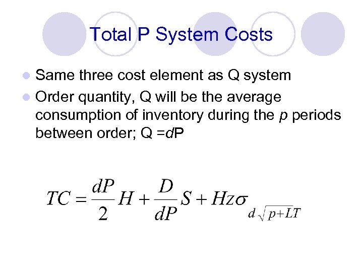
Total P System Costs Same three cost element as Q system l Order quantity, Q will be the average consumption of inventory during the p periods between order; Q =d. P l
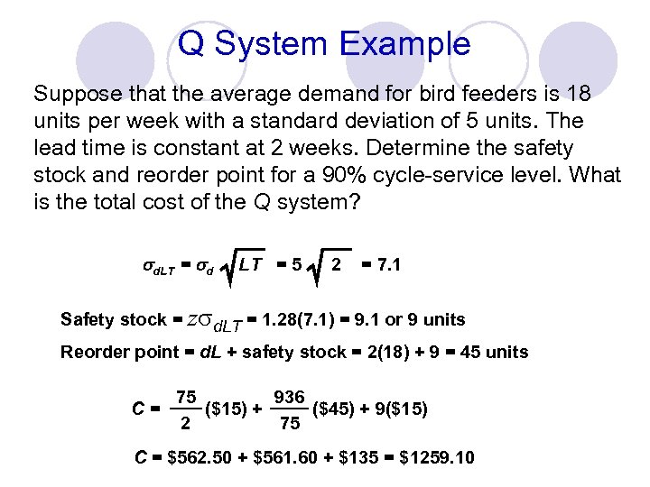
Q System Example Suppose that the average demand for bird feeders is 18 units per week with a standard deviation of 5 units. The lead time is constant at 2 weeks. Determine the safety stock and reorder point for a 90% cycle-service level. What is the total cost of the Q system? sd. LT = sd LT = 5 2 = 7. 1 Safety stock = zsd. LT = 1. 28(7. 1) = 9. 1 or 9 units Reorder point = d. L + safety stock = 2(18) + 9 = 45 units C= 75 936 ($15) + ($45) + 9($15) 2 75 C = $562. 50 + $561. 60 + $135 = $1259. 10
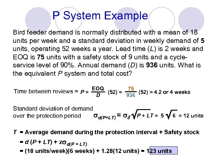
P System Example Bird feeder demand is normally distributed with a mean of 18 units per week and a standard deviation in weekly demand of 5 units, operating 52 weeks a year. Lead time (L) is 2 weeks and EOQ is 75 units with a safety stock of 9 units and a cycleservice level of 90%. Annual demand (D) is 936 units. What is the equivalent P system and total cost? Time between reviews = P = EOQ (52) = 75 (52) = 4. 2 or 4 weeks D Standard deviation of demand d(P+LT) = over the protection period 936 d P + LT = 5 6 = 12 units T = Average demand during the protection interval + Safety stock = d (P + LT) + z d(P + LT) = (18 units/week)(6 weeks) + 1. 28(12 units) = 123 units
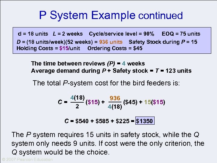
P System Example continued d = 18 units L = 2 weeks Cycle/service level = 90% EOQ = 75 units D = (18 units/week)(52 weeks) = 936 units Safety Stock during P = 15 Holding Costs = $15/unit Ordering Costs = $45 The time between reviews (P) = 4 weeks Average demand during P + Safety stock = T = 123 units The total P-system cost for the bird feeders is: 4(18) 936 C= ($15) + ($45) + 15($15) 2 4(18) C = $540 + $585 + $225 = $1350 The P system requires 15 units in safety stock, while the Q system only needs 9 units. If cost were the only criterion, the Q system would be the choice. © 2007 Pearson Education
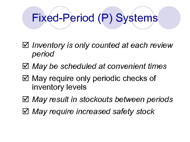
Fixed-Period (P) Systems þ Inventory is only counted at each review period þ May be scheduled at convenient times þ May require only periodic checks of inventory levels þ May result in stockouts between periods þ May require increased safety stock
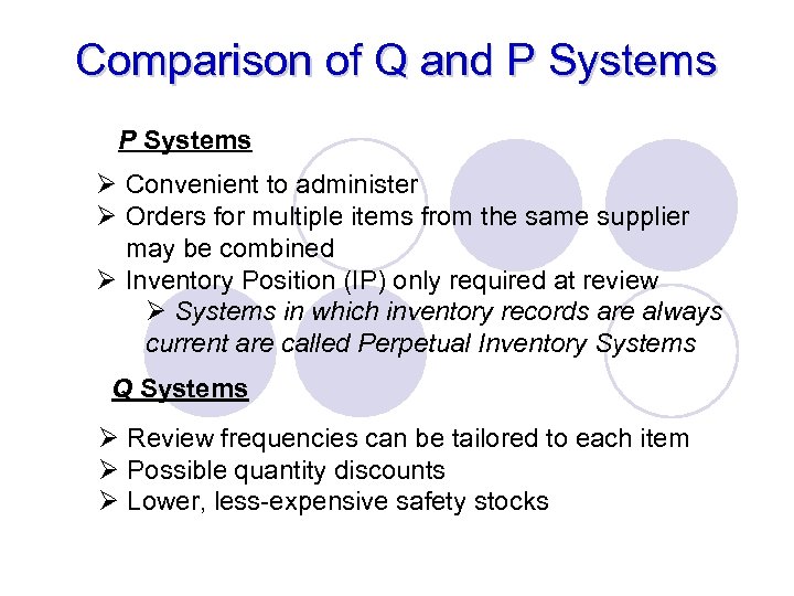
Comparison of Q and P Systems Ø Convenient to administer Ø Orders for multiple items from the same supplier may be combined Ø Inventory Position (IP) only required at review Ø Systems in which inventory records are always current are called Perpetual Inventory Systems Q Systems Ø Review frequencies can be tailored to each item Ø Possible quantity discounts Ø Lower, less-expensive safety stocks
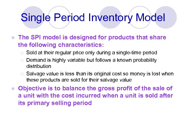
Single Period Inventory Model l The SPI model is designed for products that share the following characteristics: ¡ ¡ ¡ l Sold at their regular price only during a single-time period Demand is highly variable but follows a known probability distribution Salvage value is less than its original cost so money is lost when these products are sold for their salvage value Objective is to balance the gross profit of the sale of a unit with the cost incurred when a unit is sold after its primary selling period
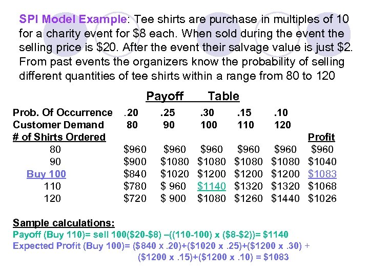
SPI Model Example: Tee shirts are purchase in multiples of 10 for a charity event for $8 each. When sold during the event the selling price is $20. After the event their salvage value is just $2. From past events the organizers know the probability of selling different quantities of tee shirts within a range from 80 to 120 Payoff Prob. Of Occurrence Customer Demand # of Shirts Ordered 80 90 Buy 100 110 120 . 20 80 $960 $900 $840 $780 $720 . 25 90 $960 $1080 $1020 $ 960 $ 900 Table. 30 100 $960 $1080 $1200 $1140 $1080 . 15 110 $960 $1080 $1200 $1320 $1260 . 10 120 $960 $1080 $1200 $1320 $1440 Profit $960 $1040 $1083 $1068 $1026 Sample calculations: Payoff (Buy 110)= sell 100($20 -$8) –((110 -100) x ($8 -$2))= $1140 Expected Profit (Buy 100)= ($840 X. 20)+($1020 x. 25)+($1200 x. 30) + ($1200 x. 15)+($1200 x. 10) = $1083
1f17d00e9ebe431bd1ddeb5a6ab4db7a.ppt