Chapter 4 Individual and Market Demand Topics

Chapter 4 Individual and Market Demand

Topics to be Discussed l Individual Demand l Income and Substitution Effects l Market Demand l Consumer Surplus l Network Externalities © 2005 Pearson Education, Inc. Chapter 4 2

Individual Demand l Price Changes m Using the figures developed in the previous chapter, the impact of a change in the price of food can be illustrated using indifference curves. m For each price change, we can determine how much of the good the individual would purchase given their budget lines and indifference curves © 2005 Pearson Education, Inc. Chapter 4 3

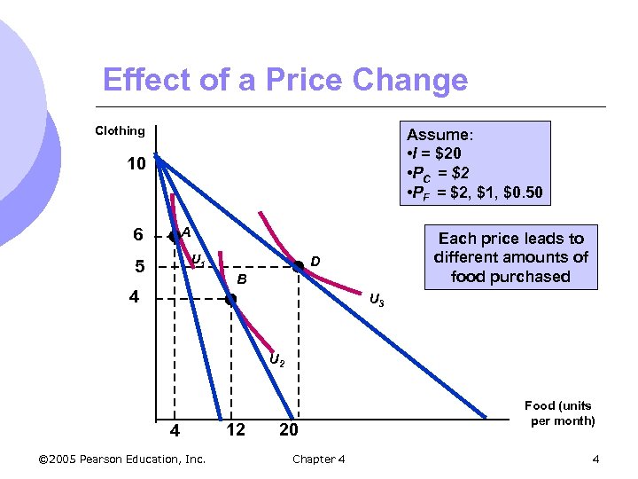Effect of a Price Change Clothing Assume: • I = $20 • PC = $2 • PF = $2, $1, $0. 50 10 A 6 U 1 5 Each price leads to different amounts of food purchased D B 4 U 3 U 2 4 © 2005 Pearson Education, Inc. 12 20 Chapter 4 Food (units per month) 4

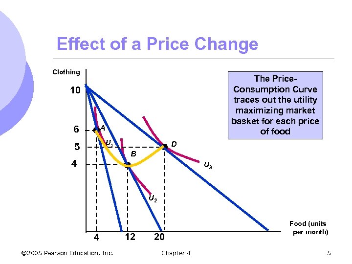Effect of a Price Change Clothing The Price. Consumption Curve traces out the utility maximizing market basket for each price of food 10 A 6 U 1 5 D B 4 U 3 U 2 4 © 2005 Pearson Education, Inc. 12 20 Chapter 4 Food (units per month) 5

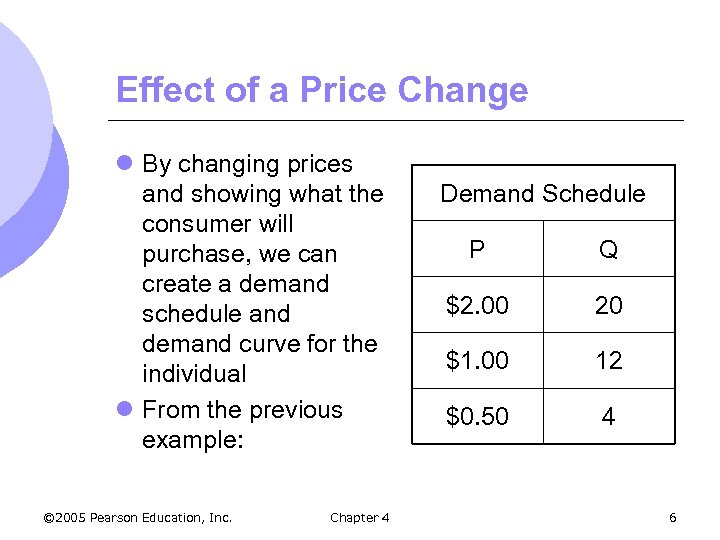Effect of a Price Change l By changing prices and showing what the consumer will purchase, we can create a demand schedule and demand curve for the individual l From the previous example: © 2005 Pearson Education, Inc. Chapter 4 Demand Schedule P Q $2. 00 20 $1. 00 12 $0. 50 4 6

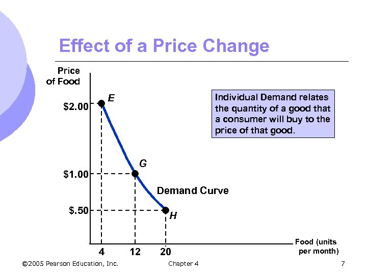Effect of a Price Change Price of Food Individual Demand relates the quantity of a good that a consumer will buy to the price of that good. E $2. 00 G $1. 00 Demand Curve $. 50 H 4 © 2005 Pearson Education, Inc. 12 20 Chapter 4 Food (units per month) 7

Demand Curves – Important Properties l The level of utility that can be attained changes as we move along the curve. l At every point on the demand curve, the consumer is maximizing utility by satisfying the condition that the MRS of food for clothing equals the ratio of the prices of food and clothing. © 2005 Pearson Education, Inc. Chapter 4 8

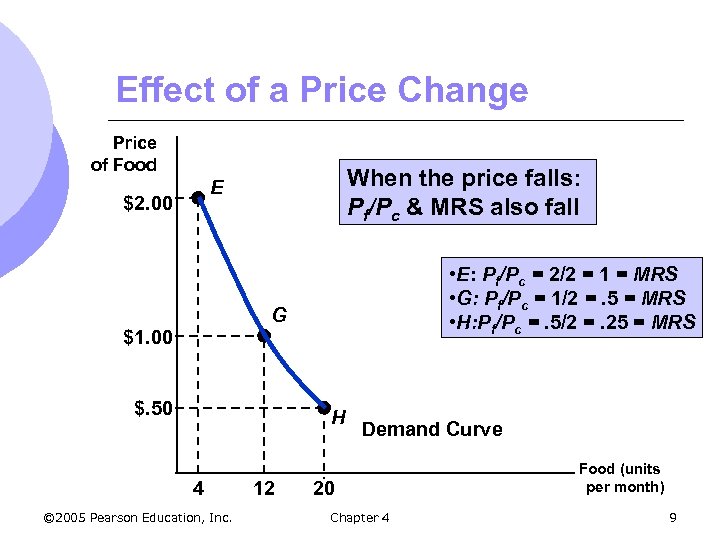Effect of a Price Change Price of Food When the price falls: Pf/Pc & MRS also fall E $2. 00 • E: Pf/Pc = 2/2 = 1 = MRS • G: Pf/Pc = 1/2 =. 5 = MRS • H: Pf/Pc =. 5/2 =. 25 = MRS G $1. 00 $. 50 H 4 © 2005 Pearson Education, Inc. 12 Demand Curve 20 Chapter 4 Food (units per month) 9

Individual Demand l Income Changes m Using the figures developed in the previous chapter, the impact of a change in the income can be illustrated using indifference curves. m Changing income, with prices fixed, causes consumer to change their market baskets. © 2005 Pearson Education, Inc. Chapter 4 10

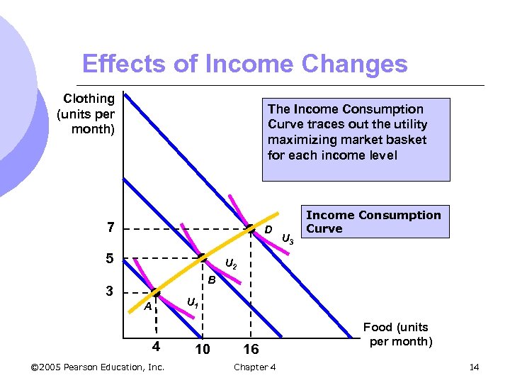
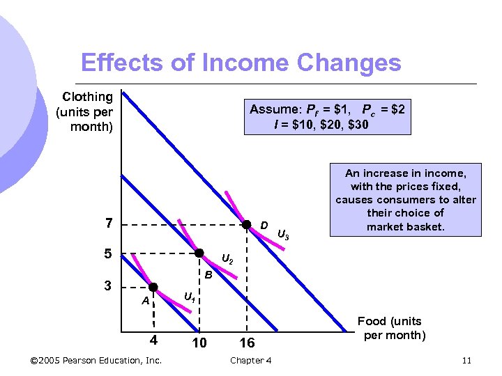Effects of Income Changes Clothing (units per month) Assume: Pf = $1, Pc = $2 I = $10, $20, $30 7 D 5 U 3 An increase in income, with the prices fixed, causes consumers to alter their choice of market basket. U 2 B 3 U 1 A 4 © 2005 Pearson Education, Inc. 10 16 Chapter 4 Food (units per month) 11

Individual Demand l Income Changes m The income-consumption curve traces out the utility-maximizing combinations of food and clothing associated with every income level. © 2005 Pearson Education, Inc. Chapter 4 12

Individual Demand l Income Changes m An increase in income shifts the budget line to the right, increasing consumption along the income-consumption curve. m Simultaneously, the increase in income shifts the demand curve to the right. © 2005 Pearson Education, Inc. Chapter 4 13

Effects of Income Changes Clothing (units per month) The Income Consumption Curve traces out the utility maximizing market basket for each income level 7 D 5 U 3 Income Consumption Curve U 2 B 3 U 1 A 4 © 2005 Pearson Education, Inc. 10 16 Chapter 4 Food (units per month) 14

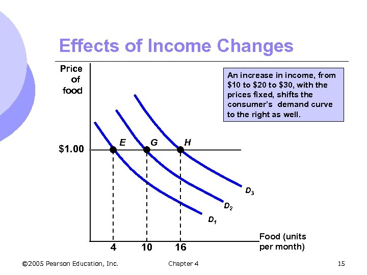Effects of Income Changes Price of food An increase in income, from $10 to $20 to $30, with the prices fixed, shifts the consumer’s demand curve to the right as well. E $1. 00 G H D 3 D 2 D 1 4 © 2005 Pearson Education, Inc. 10 16 Chapter 4 Food (units per month) 15

Individual Demand l Income Changes m When the income-consumption curve has a positive slope: l The quantity demanded increases with income. l The income elasticity of demand is positive. l The good is a normal good. © 2005 Pearson Education, Inc. Chapter 4 16

Individual Demand l Income Changes m When the income-consumption curve has a negative slope: l The quantity demanded decreases with income. l The income elasticity of demand is negative. l The good is an inferior good. © 2005 Pearson Education, Inc. Chapter 4 17

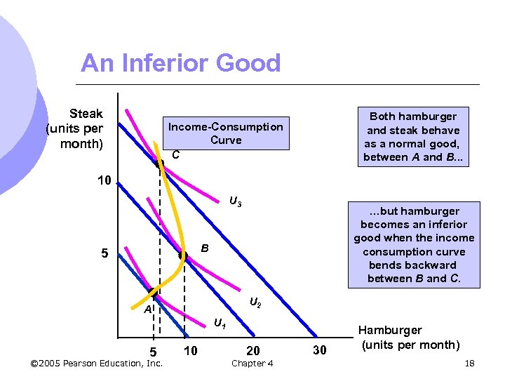An Inferior Good Steak (units per month) Both hamburger and steak behave as a normal good, between A and B. . . Income-Consumption Curve C 10 U 3 …but hamburger becomes an inferior good when the income consumption curve bends backward between B and C. B 5 U 2 A U 1 5 © 2005 Pearson Education, Inc. 10 20 Chapter 4 30 Hamburger (units per month) 18

Individual Demand l Engel Curves m Engel curves relate the quantity of good consumed to income. m If the good is a normal good, the Engel curve is upward sloping. m If the good is an inferior good, the Engel curve is downward sloping. © 2005 Pearson Education, Inc. Chapter 4 19

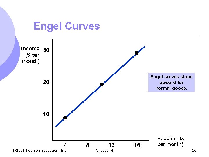Engel Curves Income 30 ($ per month) Engel curves slope upward for normal goods. 20 10 4 © 2005 Pearson Education, Inc. 8 12 Chapter 4 16 Food (units per month) 20

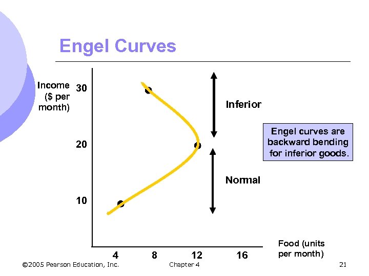Engel Curves Income 30 ($ per month) Inferior Engel curves are backward bending for inferior goods. 20 Normal 10 4 © 2005 Pearson Education, Inc. 8 12 Chapter 4 16 Food (units per month) 21

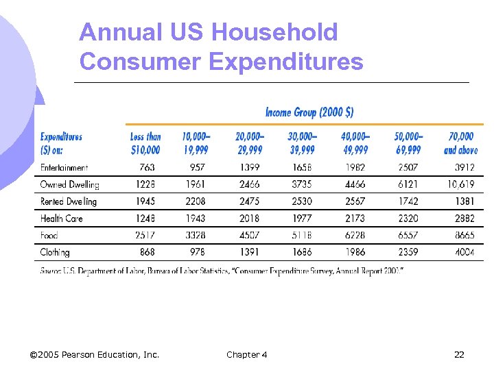Annual US Household Consumer Expenditures © 2005 Pearson Education, Inc. Chapter 4 22

Substitutes & Complements l Two goods are considered substitutes if an increase (decrease) in the price of one leads to an increase (decrease) in the quantity demanded of the other. m Ex: movie tickets and video rentals © 2005 Pearson Education, Inc. Chapter 4 23

Substitutes & Complements l Two goods are considered complements if an increase (decrease) in the price of one leads to a decrease (increase) in the quantity demanded of the other. m Ex: gasoline and motor oil © 2005 Pearson Education, Inc. Chapter 4 24

Substitutes & Complements l Two goods are independent then a change in the price of one good has no effect on the quantity demanded of the other m Ex: chicken and airplane tickets © 2005 Pearson Education, Inc. Chapter 4 25

Substitutes & Complements l If the price consumption curve is downward-sloping, the two goods are considered substitutes. l If the price consumption curve is upwardsloping, the two goods are considered complements. l They could be both. © 2005 Pearson Education, Inc. Chapter 4 26

Income and Substitution Effects l A change in the price of a good has two effects: m Substitution Effect m Income Effect © 2005 Pearson Education, Inc. Chapter 4 27

Income and Substitution Effects l Substitution Effect m Relative price of a good changes when price changes m Consumers will tend to buy more of the good that has become relatively cheaper, and less of the good that is relatively more expensive. © 2005 Pearson Education, Inc. Chapter 4 28

Income and Substitution Effects l Income Effect m Consumers experience an increase in real purchasing power when the price of one good falls. © 2005 Pearson Education, Inc. Chapter 4 29

Income and Substitution Effects l Substitution Effect m The substitution effect is the change in a good’s consumption associated with a change in the price of the good, with the level of utility held constant. m When the price of an item declines, the substitution effect always leads to an increase in the quantity demanded of the good. © 2005 Pearson Education, Inc. Chapter 4 30

Income and Substitution Effects l Income Effect m The income effect is the change in an item’s consumption brought about by the increase in purchasing power, with the price of the item held constant. m When a person’s income increases, the quantity demanded for the product may increase or decrease. © 2005 Pearson Education, Inc. Chapter 4 31

Income and Substitution Effects l Income Effect m Even with inferior goods, the income effect is rarely large enough to outweigh the substitution effect. © 2005 Pearson Education, Inc. Chapter 4 32

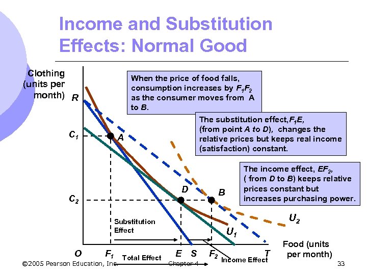Income and Substitution Effects: Normal Good Clothing (units per month) R When the price of food falls, consumption increases by F 1 F 2 as the consumer moves from A to B. The substitution effect, F 1 E, (from point A to D), changes the A relative prices but keeps real income (satisfaction) constant. C 1 D C 2 B U 2 Substitution Effect O F 1 © 2005 Pearson Education, Inc. Total Effect The income effect, EF 2, ( from D to B) keeps relative prices constant but increases purchasing power. U 1 E S Chapter 4 F 2 T Income Effect Food (units per month) 33

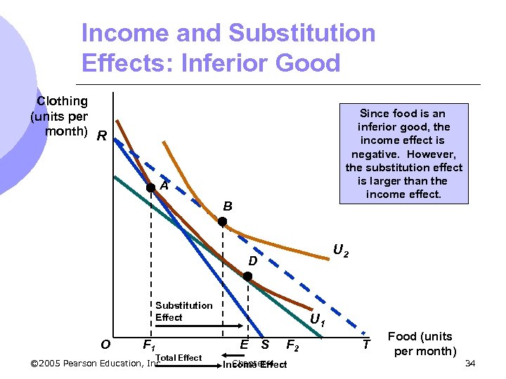Income and Substitution Effects: Inferior Good Clothing (units per month) R Since food is an inferior good, the income effect is negative. However, the substitution effect is larger than the income effect. A B U 2 D Substitution Effect O F 1 Total Effect © 2005 Pearson Education, Inc. U 1 E S F 2 Chapter 4 Income Effect T Food (units per month) 34

Income and Substitution Effects l A Special Case--The Giffen Good m The income effect may theoretically be large enough to cause the demand curve for a good to slope upward. m This rarely occurs and is of little practical interest. © 2005 Pearson Education, Inc. Chapter 4 35

Market Demand l Market Demand Curves m. A curve that relates the quantity of a good that all consumers in a market buy to the price of that good. m The sum of all the individual demand curves in the market © 2005 Pearson Education, Inc. Chapter 4 36

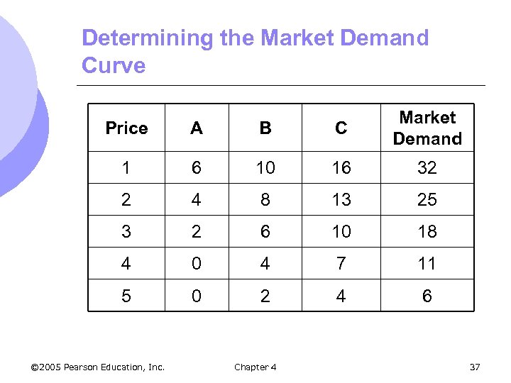Determining the Market Demand Curve Price A B C Market Demand 1 6 10 16 32 2 4 8 13 25 3 2 6 10 18 4 0 4 7 11 5 0 2 4 6 © 2005 Pearson Education, Inc. Chapter 4 37

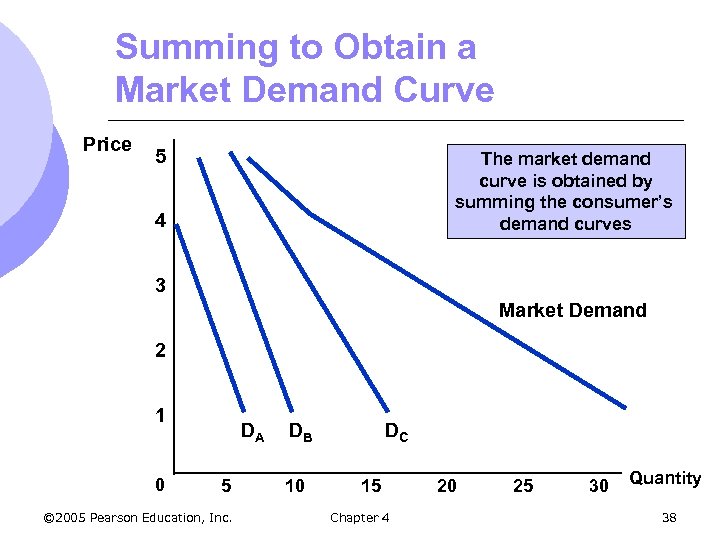Summing to Obtain a Market Demand Curve Price 5 The market demand curve is obtained by summing the consumer’s demand curves 4 3 Market Demand 2 1 0 DA 5 © 2005 Pearson Education, Inc. DB 10 DC 15 Chapter 4 20 25 30 Quantity 38

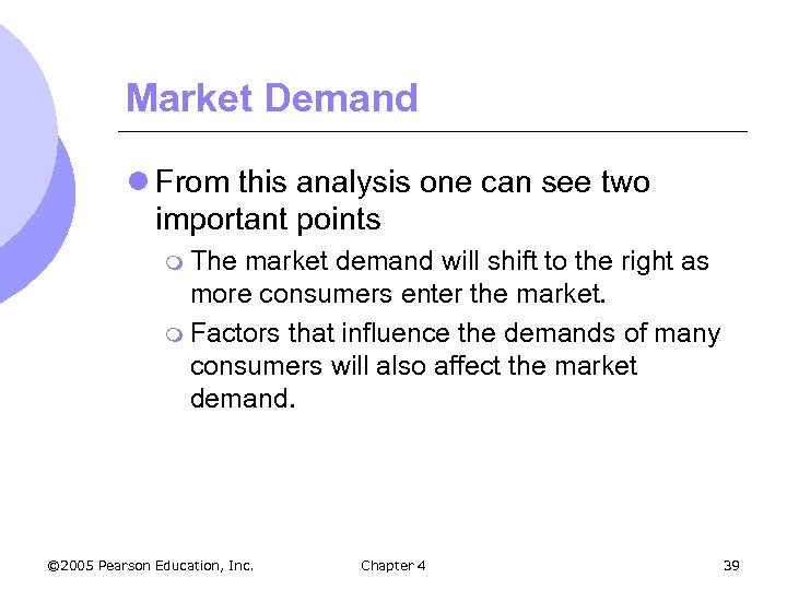Market Demand l From this analysis one can see two important points m The market demand will shift to the right as more consumers enter the market. m Factors that influence the demands of many consumers will also affect the market demand. © 2005 Pearson Education, Inc. Chapter 4 39

Market Demand l Aggregation is important to be able to discuss demand for different groups m Households with children m Consumers aged 20 – 30, etc. © 2005 Pearson Education, Inc. Chapter 4 40

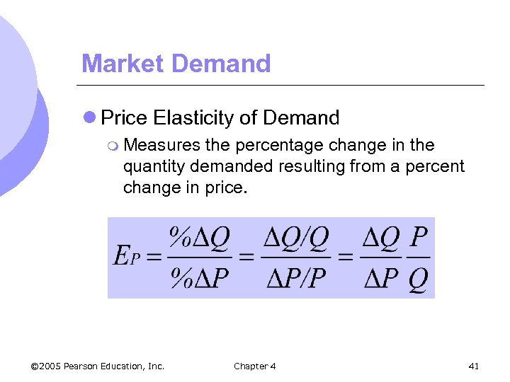Market Demand l Price Elasticity of Demand m Measures the percentage change in the quantity demanded resulting from a percent change in price. © 2005 Pearson Education, Inc. Chapter 4 41

Price Elasticity of Demand l Inelastic Demand m Ep is less than 1 in absolute value m Quantity demanded is relative unresponsive to a change in price m % Q < % P m Total expenditure (P*Q) increases when price increases © 2005 Pearson Education, Inc. Chapter 4 42

Price Elasticity of Demand l Elastic Demand m Ep is greater than 1 in absolute value m Quantity demanded is relative responsive to a change in price m % Q > % P m Total expenditure (P*Q) decreases when price increases © 2005 Pearson Education, Inc. Chapter 4 43

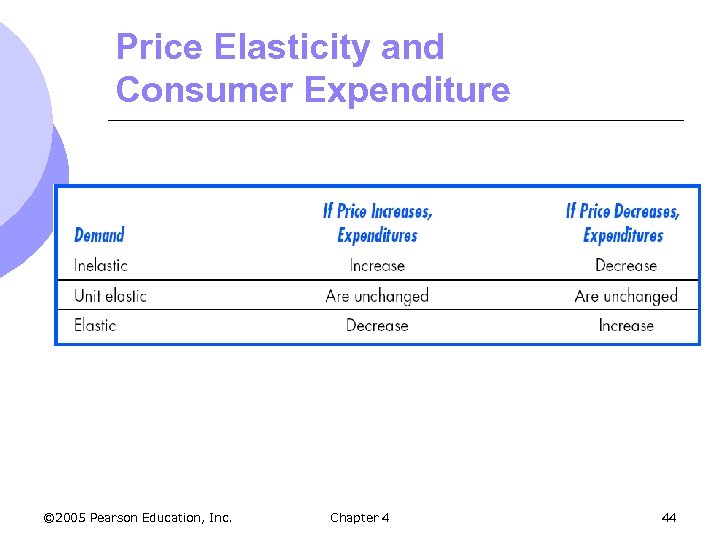Price Elasticity and Consumer Expenditure © 2005 Pearson Education, Inc. Chapter 4 44

Price Elasticity of Demand l Isoelastic Demand m When price elasticity of demand is constant along the entire demand curve m Demand curve is bowed inward (not linear) © 2005 Pearson Education, Inc. Chapter 4 45

The Aggregate Demand For Wheat l The demand for U. S. wheat is comprised of two components m Domestic demand m Export demand l Total demand for wheat can be obtained by aggregating these two demands © 2005 Pearson Education, Inc. Chapter 4 46

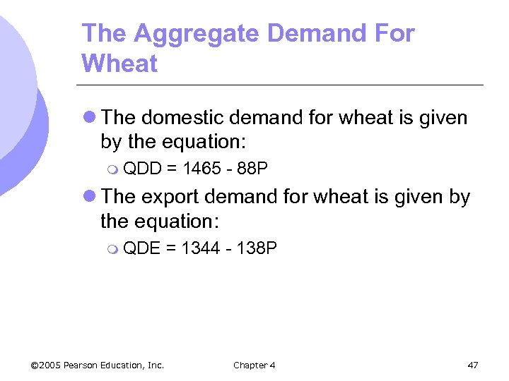The Aggregate Demand For Wheat l The domestic demand for wheat is given by the equation: m QDD = 1465 - 88 P l The export demand for wheat is given by the equation: m QDE © 2005 Pearson Education, Inc. = 1344 - 138 P Chapter 4 47

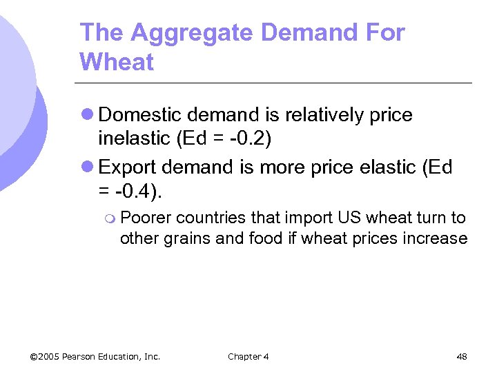The Aggregate Demand For Wheat l Domestic demand is relatively price inelastic (Ed = -0. 2) l Export demand is more price elastic (Ed = -0. 4). m Poorer countries that import US wheat turn to other grains and food if wheat prices increase © 2005 Pearson Education, Inc. Chapter 4 48

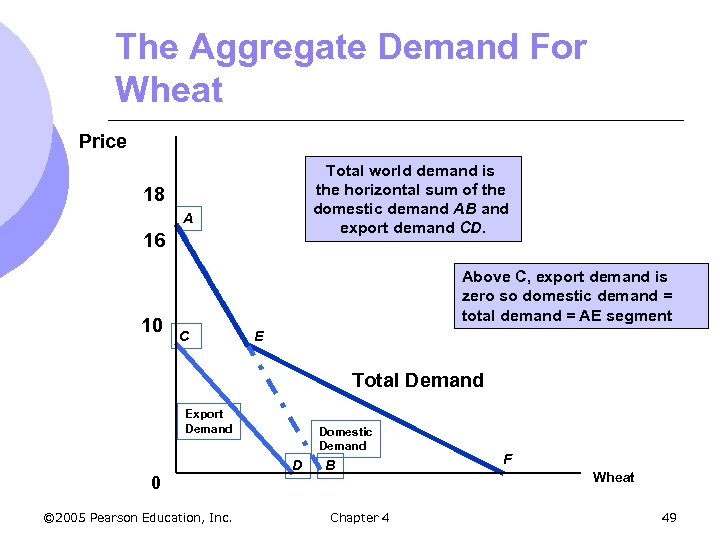The Aggregate Demand For Wheat Price Total world demand is the horizontal sum of the domestic demand AB and export demand CD. 18 A 16 10 Above C, export demand is zero so domestic demand = total demand = AE segment C E Total Demand Export Demand 0 © 2005 Pearson Education, Inc. Domestic Demand D B Chapter 4 F Wheat 49

Consumer Surplus l Consumers buy goods because it makes them better off l Consumer Surplus measures how much better off they are © 2005 Pearson Education, Inc. Chapter 4 50

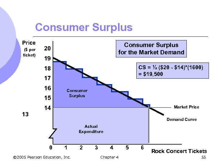
Consumer Surplus l Consumer Surplus m The difference between the maximum amount a consumer is willing to pay for a good and the amount actually paid. m Can calculate consumer surplus from the demand curve © 2005 Pearson Education, Inc. Chapter 4 51

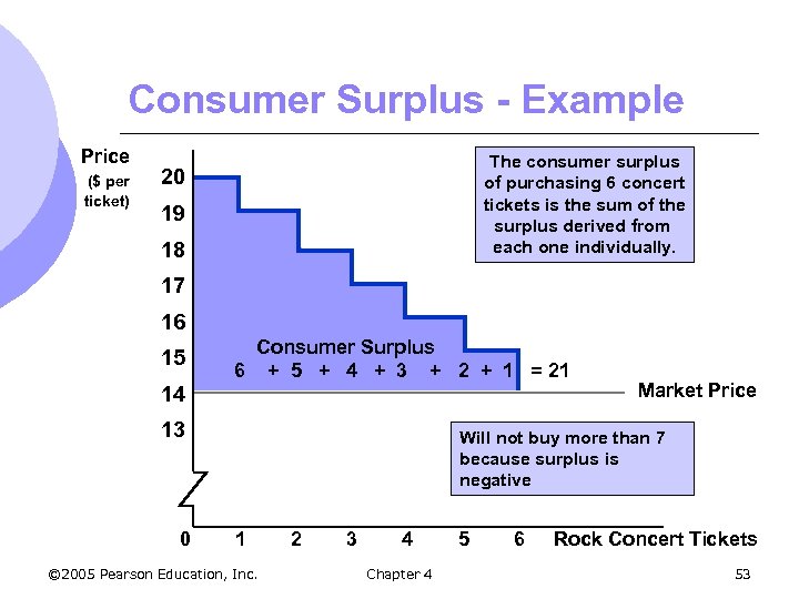
Consumer Surplus - Example l Student wants to buy concert tickets l Demand curve tells us willingness to pay for each concert ticket m 1 st ticket worth $20 but price is $14 so student generates $6 worth of surplus m Can measure this for each ticket m Total surplus is addition of surplus for each ticket purchased © 2005 Pearson Education, Inc. Chapter 4 52

Consumer Surplus - Example Price ($ per ticket) The consumer surplus of purchasing 6 concert tickets is the sum of the surplus derived from each one individually. 20 19 18 17 16 15 14 Consumer Surplus 6 + 5 + 4 + 3 + 2 + 1 = 21 13 0 Market Price Will not buy more than 7 because surplus is negative 1 © 2005 Pearson Education, Inc. 2 3 4 Chapter 4 5 6 Rock Concert Tickets 53

Consumer Surplus l The stepladder demand curve can be converted into a straight-line demand curve by making the units of the good smaller. l Consumer surplus is area under the demand curve and above the price © 2005 Pearson Education, Inc. Chapter 4 54

Consumer Surplus Price ($ per ticket) Consumer Surplus for the Market Demand 20 19 CS = ½ ($20 - $14)*(1600) = $19, 500 18 17 16 15 13 Consumer Surplus 14 Market Price Demand Curve Actual Expenditure 0 1 © 2005 Pearson Education, Inc. 2 3 4 Chapter 4 5 6 Rock Concert Tickets 55

Applying Consumer Surplus l Combining consumer surplus with the aggregate profits that producers obtain we can evaluate: 1. 2. Costs and benefits of different market structures Public policies that alter the behavior of consumers and firms © 2005 Pearson Education, Inc. Chapter 4 56

Applying Consumer Surplus – An Example l The Value of Clean Air m Air is free in the sense that we don’t pay to breathe it. m The Clean Air Act was amended in 1970. m Question: Were the benefits of cleaning up the air worth the costs? © 2005 Pearson Education, Inc. Chapter 4 57

The Value of Clean Air l Empirical data determined estimates for the demand for clean air l No market exists for clean air, but can see people are willing to pay for it m Ex: People pay more to buy houses where the air is clean. © 2005 Pearson Education, Inc. Chapter 4 58

The Value of Cleaner Air l Using these empirical estimates, we can measure people’s consumer surplus for pollution reduction from the demand curve © 2005 Pearson Education, Inc. Chapter 4 59

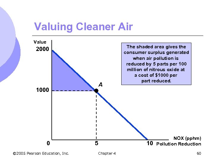Valuing Cleaner Air Value 2000 A 1000 0 © 2005 Pearson Education, Inc. 5 The shaded area gives the consumer surplus generated when air pollution is reduced by 5 parts per 100 million of nitrous oxide at a cost of $1000 per part reduced. 10 Chapter 4 NOX (pphm) Pollution Reduction 60

Value of Cleaner Air l A full cost-benefit analysis would include total benefit of cleanup l Total benefits would be compared to total costs to determine if the clean up was worth while © 2005 Pearson Education, Inc. Chapter 4 61

Network Externalities l Up to this point we have assumed that people’s demands for a good are independent of one another. l For some goods, one person’s demand also depends on the demands of other people © 2005 Pearson Education, Inc. Chapter 4 62

Network Externalities l If this is the case, a network externality exists. l Network externalities can be positive or negative. © 2005 Pearson Education, Inc. Chapter 4 63

Network Externalities l A positive network externality exists if the quantity of a good demanded by a consumer increases in response to an increase in purchases by other consumers. l Negative network externalities are just the opposite. © 2005 Pearson Education, Inc. Chapter 4 64

Network Externalities l The Bandwagon Effect m This is the desire to be in style, to have a good because almost everyone else has it, or to indulge in a fad. m This is the major objective of marketing and advertising campaigns (e. g. toys, clothing). m Positive network externality in which a consumer wishes to possess a good in part because others do © 2005 Pearson Education, Inc. Chapter 4 65

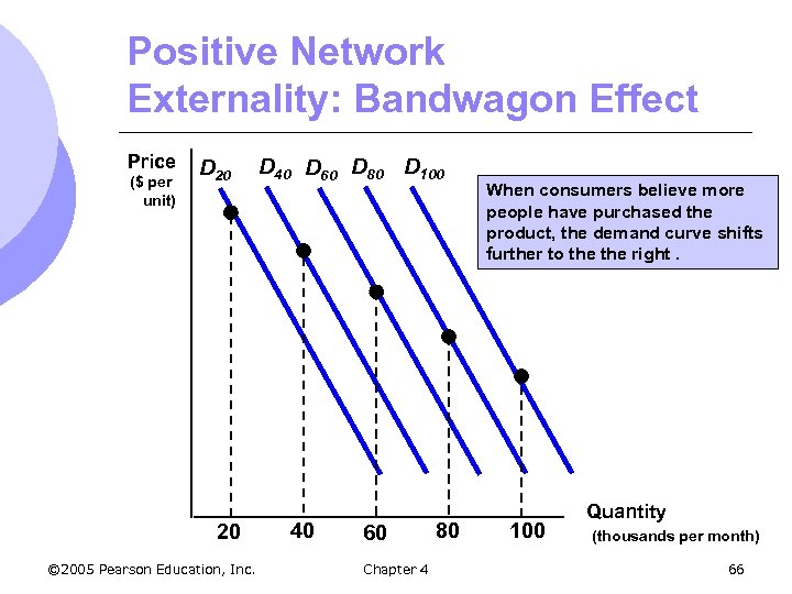Positive Network Externality: Bandwagon Effect Price ($ per unit) D 20 20 © 2005 Pearson Education, Inc. D 40 D 60 D 80 D 100 40 60 Chapter 4 80 When consumers believe more people have purchased the product, the demand curve shifts further to the right. 100 Quantity (thousands per month) 66

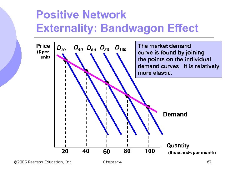Positive Network Externality: Bandwagon Effect Price ($ per unit) D 20 D 40 D 60 D 80 D 100 The market demand curve is found by joining the points on the individual demand curves. It is relatively more elastic. Demand 20 © 2005 Pearson Education, Inc. 40 60 Chapter 4 80 100 Quantity (thousands per month) 67

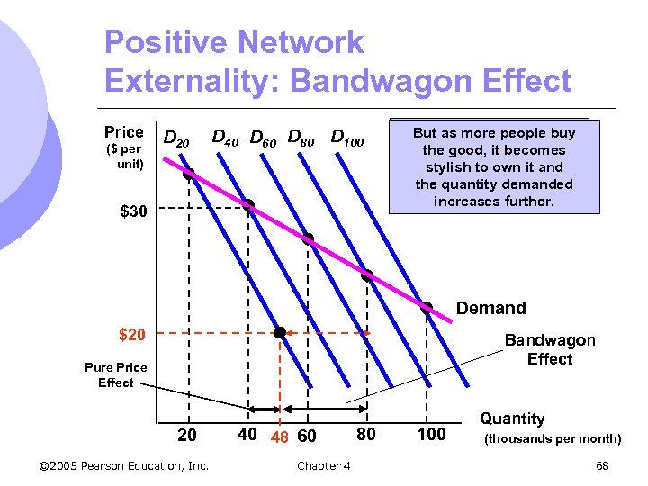Positive Network Externality: Bandwagon Effect Price ($ per unit) D 20 D 40 D 60 D 80 D 100 $30 Suppose more people buy But as the price falls from $30 to $20. becomes the good, it If there were no bandwagon and stylish to own it effect, quantity demanded would the quantity demanded only increase tofurther. increases 48, 000 Demand $20 Bandwagon Effect Pure Price Effect 20 © 2005 Pearson Education, Inc. 40 48 60 Chapter 4 80 100 Quantity (thousands per month) 68

Network Externalities l The Snob Effect m If the network externality is negative, a snob effect exists. l The snob effect refers to the desire to own exclusive or unique goods. l The quantity demanded of a “snob” good is higher the fewer the people who own it. © 2005 Pearson Education, Inc. Chapter 4 69

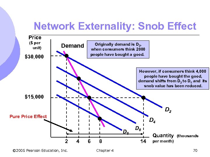Network Externality: Snob Effect Price ($ per unit) Demand $30, 000 Originally demand is D 2, when consumers think 2000 people have bought a good. However, if consumers think 4, 000 people have bought the good, demand shifts from D 2 to D 6 and its snob value has been reduced. $15, 000 D 2 Pure Price Effect D 4 D 8 2 © 2005 Pearson Education, Inc. 4 6 8 Chapter 4 D 6 14 Quantity (thousands per month) 70

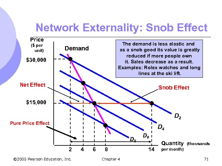Network Externality: Snob Effect Price ($ per unit) The demand is less elastic and as a snob good its value is greatly reduced if more people own it. Sales decrease as a result. Examples: Rolex watches and long lines at the ski lift. Demand $30, 000 Net Effect Snob Effect $15, 000 D 2 Pure Price Effect D 4 D 8 2 © 2005 Pearson Education, Inc. 4 6 8 Chapter 4 D 6 14 Quantity (thousands per month) 71