953a5442d04b4d460bb7eed124392894.ppt
- Количество слайдов: 41
 Chapter 4 Individual and Market Demand Slide Copyright © 2004 Mc. Graw-Hill Ryerson Limited
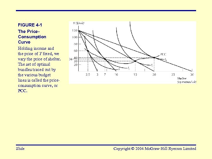 FIGURE 4 -1 The Price. Consumption Curve Holding income and the price of Y fixed, we vary the price of shelter. The set of optimal bundles traced out by the various budget lines is called the priceconsumption curve, or PCC. Slide Copyright © 2004 Mc. Graw-Hill Ryerson Limited
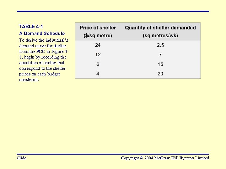 TABLE 4 -1 A Demand Schedule To derive the individual’s demand curve for shelter from the PCC in Figure 41, begin by recording the quantities of shelter that correspond to the shelter prices on each budget constraint. Slide Copyright © 2004 Mc. Graw-Hill Ryerson Limited
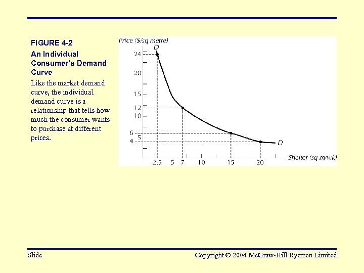 FIGURE 4 -2 An Individual Consumer’s Demand Curve Like the market demand curve, the individual demand curve is a relationship that tells how much the consumer wants to purchase at different prices. Slide Copyright © 2004 Mc. Graw-Hill Ryerson Limited
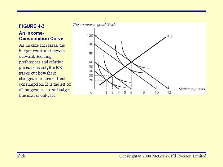 FIGURE 4 -3 An Income. Consumption Curve As income increases, the budget constraint moves outward. Holding preferences and relative prices constant, the ICC traces out how these changes in income affect consumption. It is the set of all tangencies as the budget line moves outward. Slide Copyright © 2004 Mc. Graw-Hill Ryerson Limited
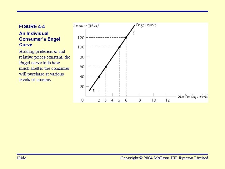 FIGURE 4 -4 An Individual Consumer’s Engel Curve Holding preferences and relative prices constant, the Engel curve tells how much shelter the consumer will purchase at various levels of income. Slide Copyright © 2004 Mc. Graw-Hill Ryerson Limited
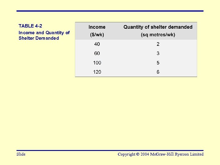 TABLE 4 -2 Income and Quantity of Shelter Demanded Slide Copyright © 2004 Mc. Graw-Hill Ryerson Limited
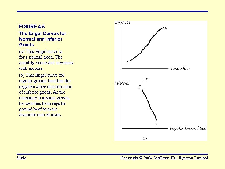 FIGURE 4 -5 The Engel Curves for Normal and Inferior Goods (a) This Engel curve is for a normal good. The quantity demanded increases with income. (b) This Engel curve for regular ground beef has the negative slope characteristic of inferior goods. As the consumer’s income grows, he switches from regular ground beef to more desirable cuts of meat. Slide Copyright © 2004 Mc. Graw-Hill Ryerson Limited
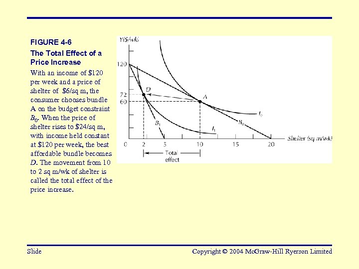 FIGURE 4 -6 The Total Effect of a Price Increase With an income of $120 per week and a price of shelter of $6/sq m, the consumer chooses bundle A on the budget constraint B 0. When the price of shelter rises to $24/sq m, with income held constant at $120 per week, the best affordable bundle becomes D. The movement from 10 to 2 sq m/wk of shelter is called the total effect of the price increase. Slide Copyright © 2004 Mc. Graw-Hill Ryerson Limited
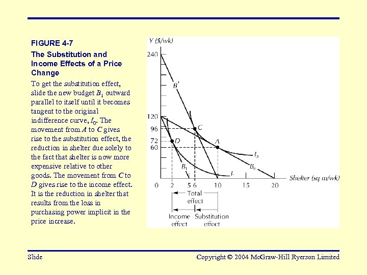 FIGURE 4 -7 The Substitution and Income Effects of a Price Change To get the substitution effect, slide the new budget B 1 outward parallel to itself until it becomes tangent to the original indifference curve, I 0. The movement from A to C gives rise to the substitution effect, the reduction in shelter due solely to the fact that shelter is now more expensive relative to other goods. The movement from C to D gives rise to the income effect. It is the reduction in shelter that results from the loss in purchasing power implicit in the price increase. Slide Copyright © 2004 Mc. Graw-Hill Ryerson Limited
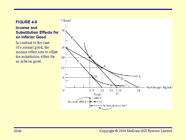 FIGURE 4 -8 Income and Substitution Effects for an Inferior Good In contrast to the case of a normal good, the income effect acts to offset the substitution effect for an inferior good. Slide Copyright © 2004 Mc. Graw-Hill Ryerson Limited
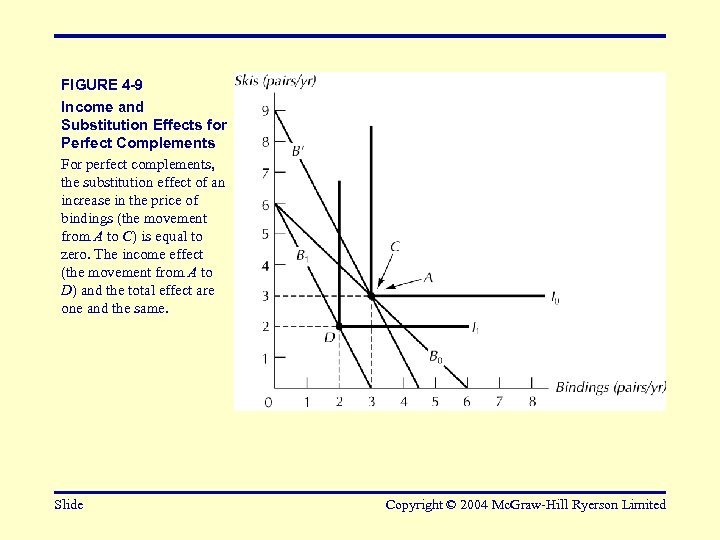 FIGURE 4 -9 Income and Substitution Effects for Perfect Complements For perfect complements, the substitution effect of an increase in the price of bindings (the movement from A to C) is equal to zero. The income effect (the movement from A to D) and the total effect are one and the same. Slide Copyright © 2004 Mc. Graw-Hill Ryerson Limited
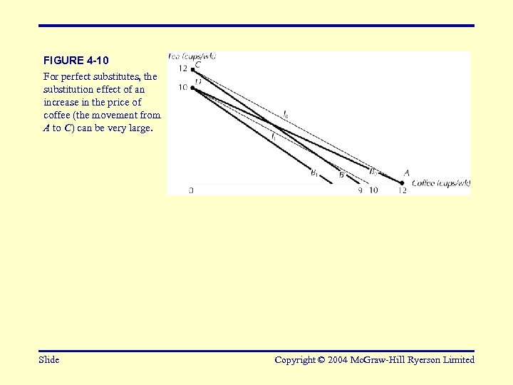 FIGURE 4 -10 For perfect substitutes, the substitution effect of an increase in the price of coffee (the movement from A to C) can be very large. Slide Copyright © 2004 Mc. Graw-Hill Ryerson Limited
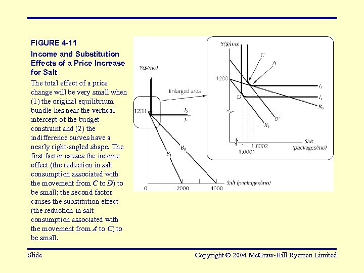 FIGURE 4 -11 Income and Substitution Effects of a Price Increase for Salt The total effect of a price change will be very small when (1) the original equilibrium bundle lies near the vertical intercept of the budget constraint and (2) the indifference curves have a nearly right-angled shape. The first factor causes the income effect (the reduction in salt consumption associated with the movement from C to D) to be small; the second factor causes the substitution effect (the reduction in salt consumption associated with the movement from A to C) to be small. Slide Copyright © 2004 Mc. Graw-Hill Ryerson Limited
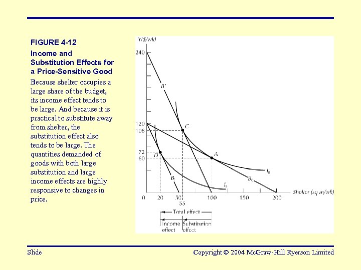 FIGURE 4 -12 Income and Substitution Effects for a Price-Sensitive Good Because shelter occupies a large share of the budget, its income effect tends to be large. And because it is practical to substitute away from shelter, the substitution effect also tends to be large. The quantities demanded of goods with both large substitution and large income effects are highly responsive to changes in price. Slide Copyright © 2004 Mc. Graw-Hill Ryerson Limited
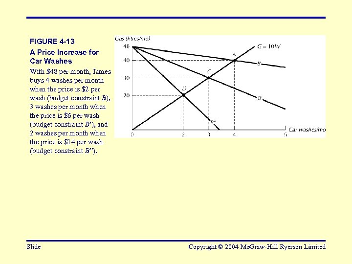 FIGURE 4 -13 A Price Increase for Car Washes With $48 per month, James buys 4 washes per month when the price is $2 per wash (budget constraint B), 3 washes per month when the price is $6 per wash (budget constraint B ), and 2 washes per month when the price is $14 per wash (budget constraint B ). Slide Copyright © 2004 Mc. Graw-Hill Ryerson Limited
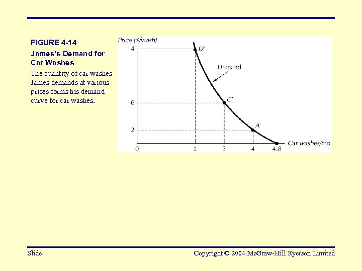 FIGURE 4 -14 James’s Demand for Car Washes The quantity of car washes James demands at various prices forms his demand curve for car washes. Slide Copyright © 2004 Mc. Graw-Hill Ryerson Limited
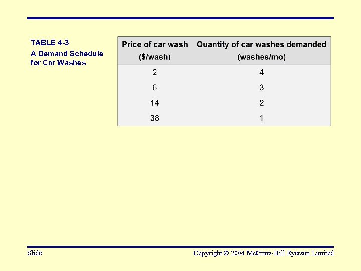 TABLE 4 -3 A Demand Schedule for Car Washes Slide Copyright © 2004 Mc. Graw-Hill Ryerson Limited
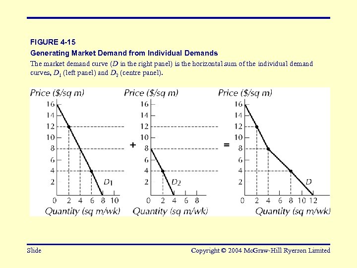 FIGURE 4 -15 Generating Market Demand from Individual Demands The market demand curve (D in the right panel) is the horizontal sum of the individual demand curves, D 1 (left panel) and D 2 (centre panel). Slide Copyright © 2004 Mc. Graw-Hill Ryerson Limited
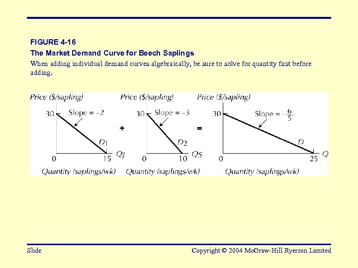 FIGURE 4 -16 The Market Demand Curve for Beech Saplings When adding individual demand curves algebraically, be sure to solve for quantity first before adding. Slide Copyright © 2004 Mc. Graw-Hill Ryerson Limited
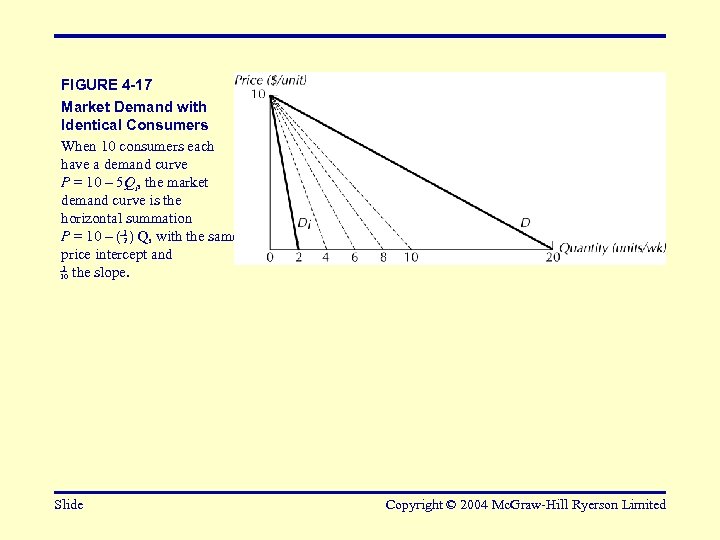 FIGURE 4 -17 Market Demand with Identical Consumers When 10 consumers each have a demand curve P = 10 – 5 Qi, the market demand curve is the horizontal summation P = 10 – ( 1 ) Q, with the same 2 price intercept and 1 10 the slope. Slide Copyright © 2004 Mc. Graw-Hill Ryerson Limited
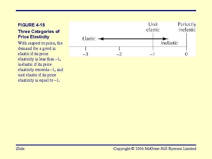 FIGURE 4 -18 Three Categories of Price Elasticity With respect to price, the demand for a good is elastic if its price elasticity is less than – 1, inelastic if its price elasticity exceeds – 1, and unit elastic if its price elasticity is equal to – 1. Slide Copyright © 2004 Mc. Graw-Hill Ryerson Limited
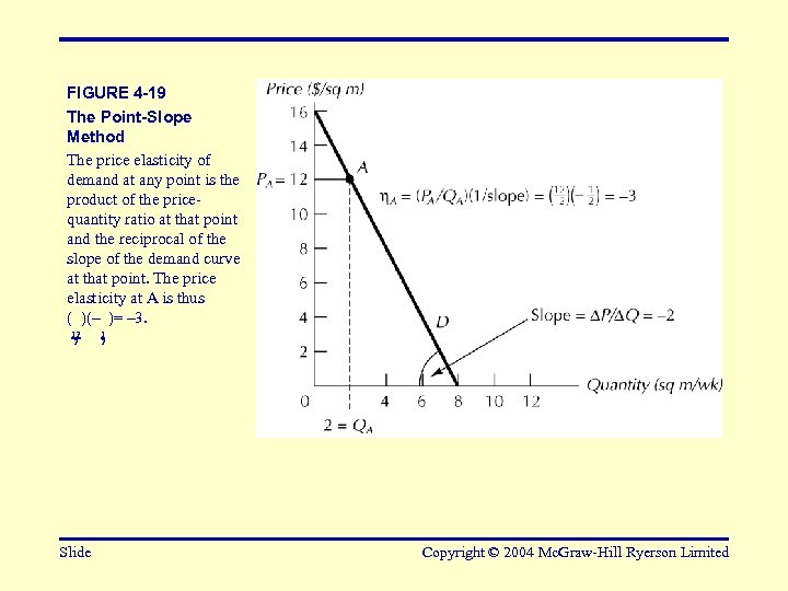 FIGURE 4 -19 The Point-Slope Method The price elasticity of demand at any point is the product of the pricequantity ratio at that point and the reciprocal of the slope of the demand curve at that point. The price elasticity at A is thus ( )(– )= – 3. 12 2 Slide 1 2 Copyright © 2004 Mc. Graw-Hill Ryerson Limited
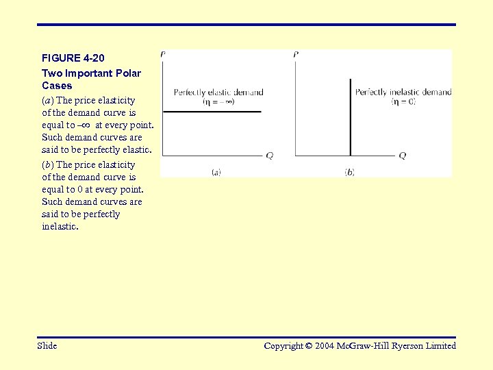 FIGURE 4 -20 Two Important Polar Cases (a) The price elasticity of the demand curve is equal to – at every point. Such demand curves are said to be perfectly elastic. (b) The price elasticity of the demand curve is equal to 0 at every point. Such demand curves are said to be perfectly inelastic. Slide Copyright © 2004 Mc. Graw-Hill Ryerson Limited
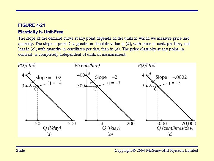 FIGURE 4 -21 Elasticity Is Unit-Free The slope of the demand curve at any point depends on the units in which we measure price and quantity. The slope at point C is greater in absolute value in (b), with price in cents per litre, and less in (c), with quantity in centilitres per day, than in (a). The price elasticity at any point, in contrast, is completely independent of units of measurement. Slide Copyright © 2004 Mc. Graw-Hill Ryerson Limited
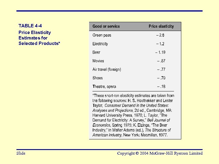 TABLE 4 -4 Price Elasticity Estimates for Selected Products* Slide Copyright © 2004 Mc. Graw-Hill Ryerson Limited
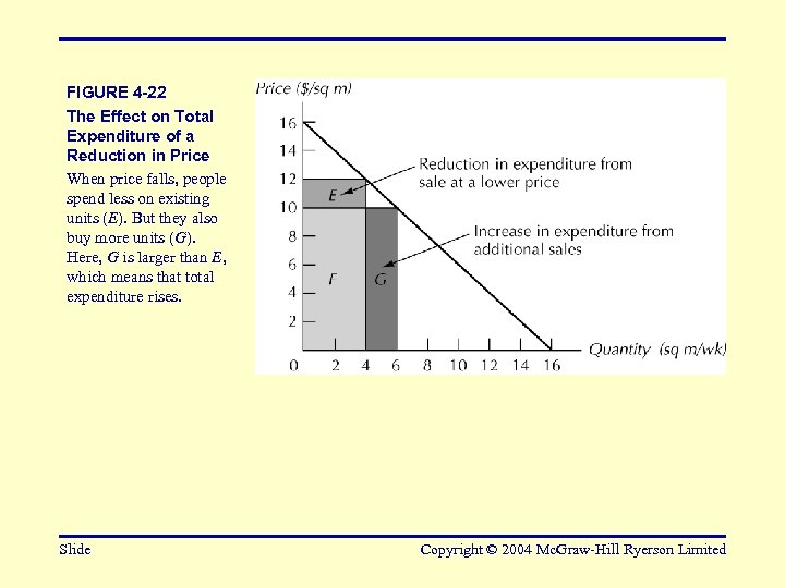 FIGURE 4 -22 The Effect on Total Expenditure of a Reduction in Price When price falls, people spend less on existing units (E). But they also buy more units (G). Here, G is larger than E, which means that total expenditure rises. Slide Copyright © 2004 Mc. Graw-Hill Ryerson Limited
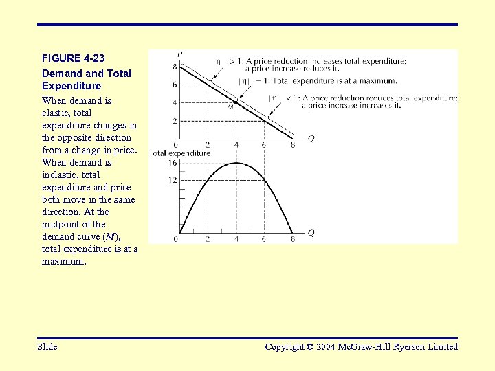 FIGURE 4 -23 Demand Total Expenditure When demand is elastic, total expenditure changes in the opposite direction from a change in price. When demand is inelastic, total expenditure and price both move in the same direction. At the midpoint of the demand curve (M), total expenditure is at a maximum. Slide Copyright © 2004 Mc. Graw-Hill Ryerson Limited
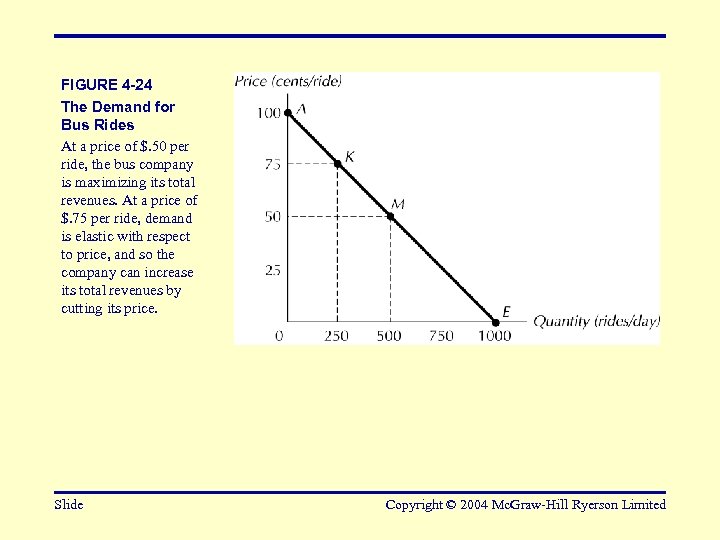 FIGURE 4 -24 The Demand for Bus Rides At a price of $. 50 per ride, the bus company is maximizing its total revenues. At a price of $. 75 per ride, demand is elastic with respect to price, and so the company can increase its total revenues by cutting its price. Slide Copyright © 2004 Mc. Graw-Hill Ryerson Limited
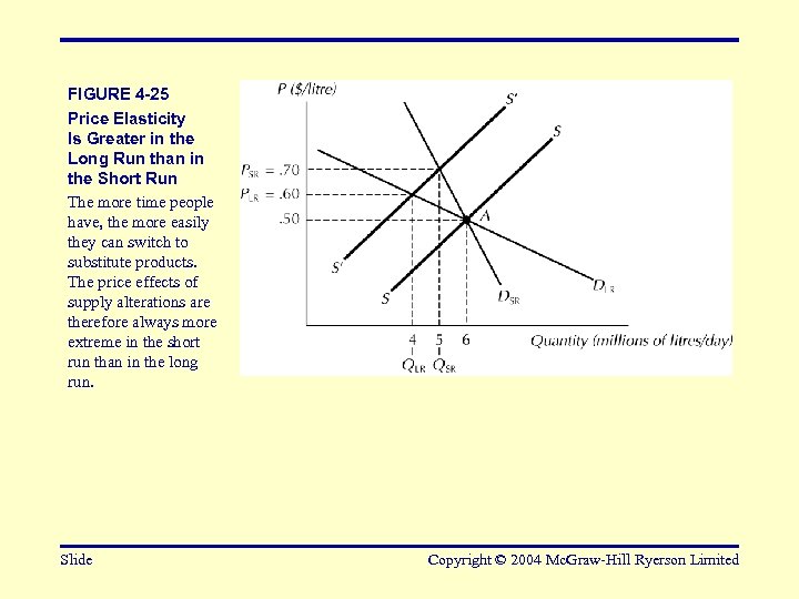 FIGURE 4 -25 Price Elasticity Is Greater in the Long Run than in the Short Run The more time people have, the more easily they can switch to substitute products. The price effects of supply alterations are therefore always more extreme in the short run than in the long run. Slide Copyright © 2004 Mc. Graw-Hill Ryerson Limited
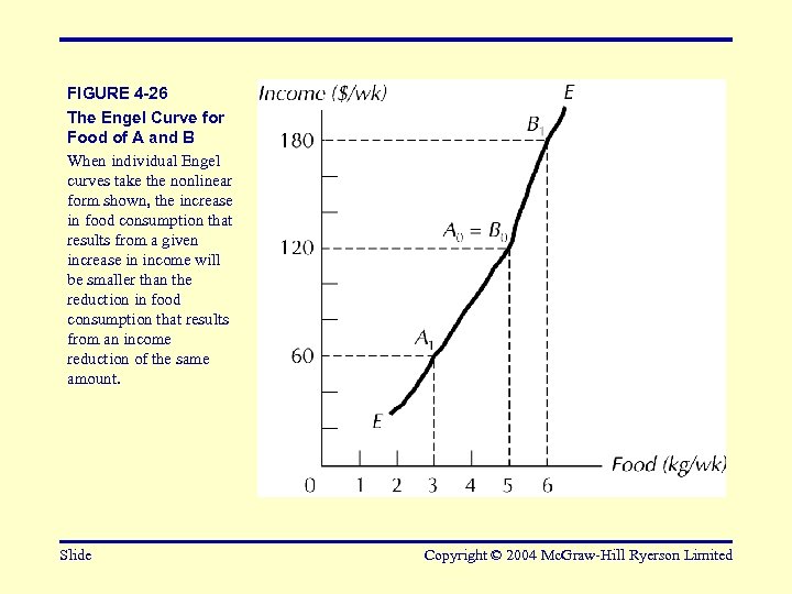 FIGURE 4 -26 The Engel Curve for Food of A and B When individual Engel curves take the nonlinear form shown, the increase in food consumption that results from a given increase in income will be smaller than the reduction in food consumption that results from an income reduction of the same amount. Slide Copyright © 2004 Mc. Graw-Hill Ryerson Limited
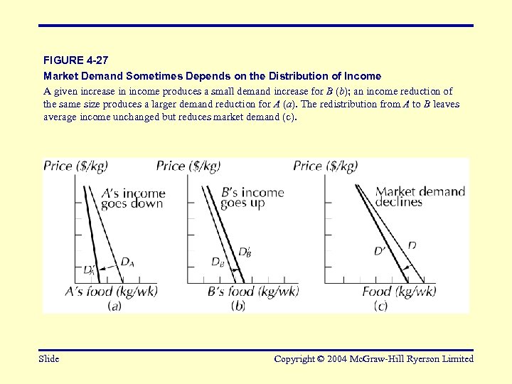 FIGURE 4 -27 Market Demand Sometimes Depends on the Distribution of Income A given increase in income produces a small demand increase for B (b); an income reduction of the same size produces a larger demand reduction for A (a). The redistribution from A to B leaves average income unchanged but reduces market demand (c). Slide Copyright © 2004 Mc. Graw-Hill Ryerson Limited
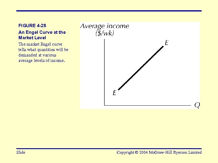 FIGURE 4 -28 An Engel Curve at the Market Level The market Engel curve tells what quantities will be demanded at various average levels of income. Slide Copyright © 2004 Mc. Graw-Hill Ryerson Limited
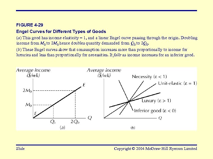 FIGURE 4 -29 Engel Curves for Different Types of Goods (a) This good has income elasticity = 1, and a linear Engel curve passing through the origin. Doubling income from M 0 to 2 M 0 hence doubles quantity demanded from Q 0 to 2 Q 0. (b) These Engel curves show that consumption increases more than proportionally to income for luxuries and less than proportionally for necessities. It falls as income increases for an inferior good. Slide Copyright © 2004 Mc. Graw-Hill Ryerson Limited
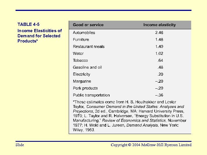 TABLE 4 -5 Income Elasticities of Demand for Selected Products* Slide Copyright © 2004 Mc. Graw-Hill Ryerson Limited
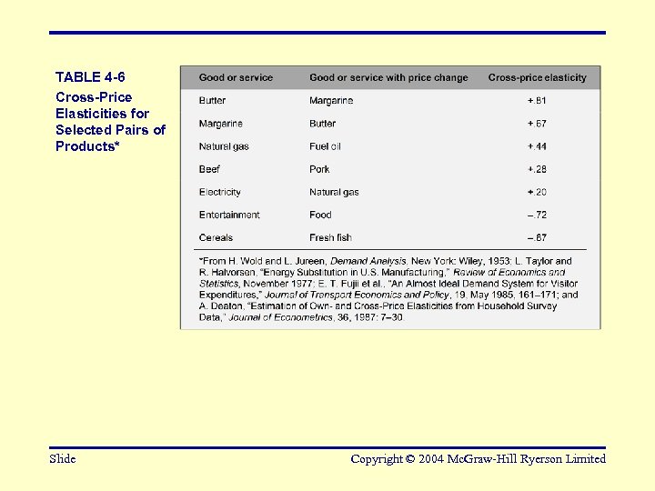 TABLE 4 -6 Cross-Price Elasticities for Selected Pairs of Products* Slide Copyright © 2004 Mc. Graw-Hill Ryerson Limited
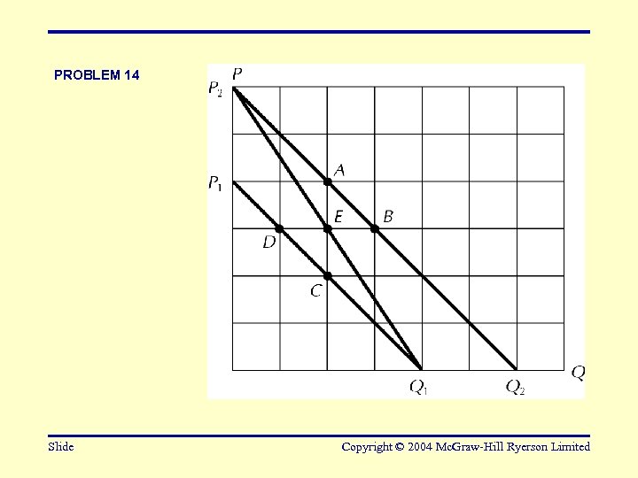 PROBLEM 14 Slide Copyright © 2004 Mc. Graw-Hill Ryerson Limited
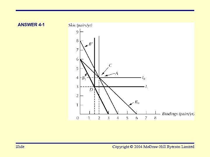 ANSWER 4 -1 Slide Copyright © 2004 Mc. Graw-Hill Ryerson Limited
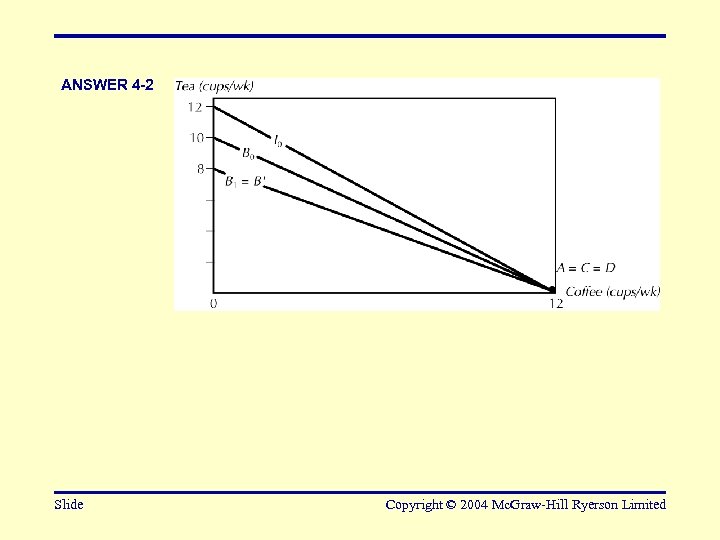 ANSWER 4 -2 Slide Copyright © 2004 Mc. Graw-Hill Ryerson Limited
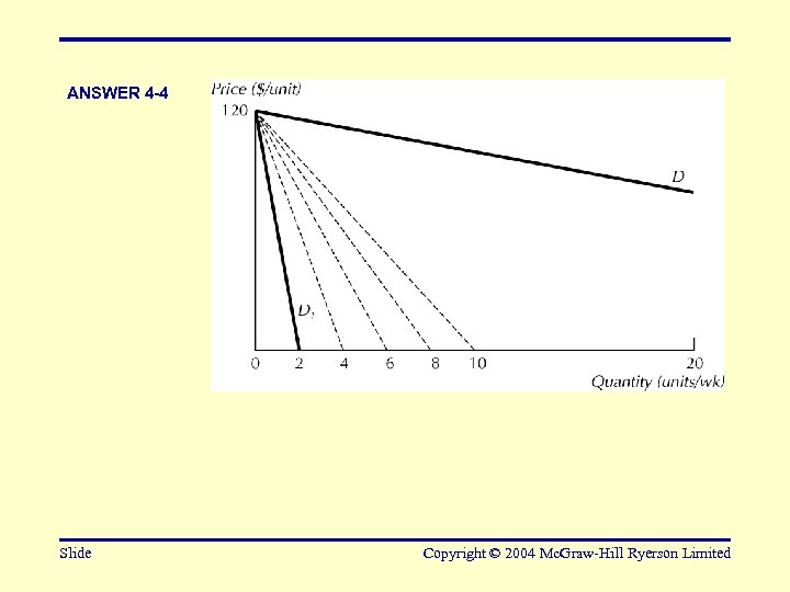 ANSWER 4 -4 Slide Copyright © 2004 Mc. Graw-Hill Ryerson Limited
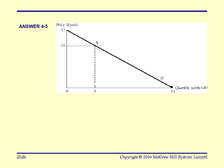 ANSWER 4 -5 Slide Copyright © 2004 Mc. Graw-Hill Ryerson Limited


