04e4a65dd8d1b0f378258d785eafe35c.ppt
- Количество слайдов: 80
Chapter 4 Describing Bivariate Numerical Data Created by Kathy Fritz
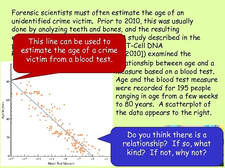
Forensic scientists must often estimate the age of an unidentified crime victim. Prior to 2010, this was usually done by analyzing teeth and bones, and the resulting estimates were not very reliable. A study described in the This line can be used to paper “Estimating Human Age from T-Cell DNA estimate the age of a crime Rearrangements” (Current Biology [2010]) examined the victim from a blood test. relationship between age and a measure based on a blood test. Age and the blood test measure were recorded for 195 people ranging in age from a few weeks to 80 years. A scatterplot of the data appears to the right. Do you think there is a relationship? If so, what kind? If not, why not?
Correlation Pearson’s Sample Correlation Coefficient Properties of r
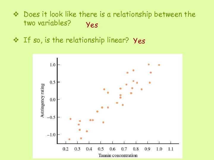
v Does it look like there is a relationship between the two variables? Yes v If so, is the relationship linear? Yes
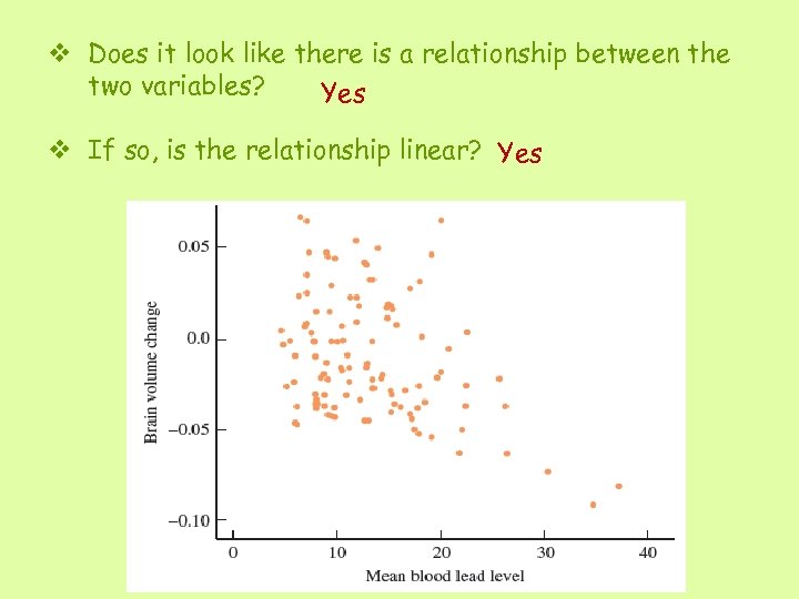
v Does it look like there is a relationship between the two variables? Yes v If so, is the relationship linear? Yes
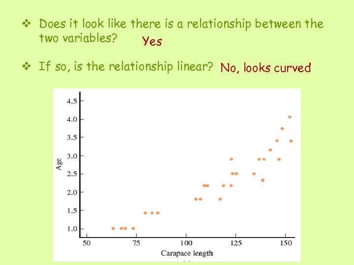
v Does it look like there is a relationship between the two variables? Yes v If so, is the relationship linear? No, looks curved
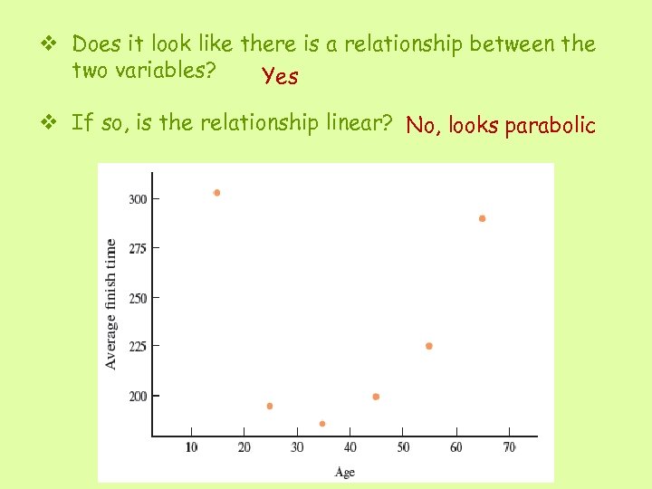
v Does it look like there is a relationship between the two variables? Yes v If so, is the relationship linear? No, looks parabolic
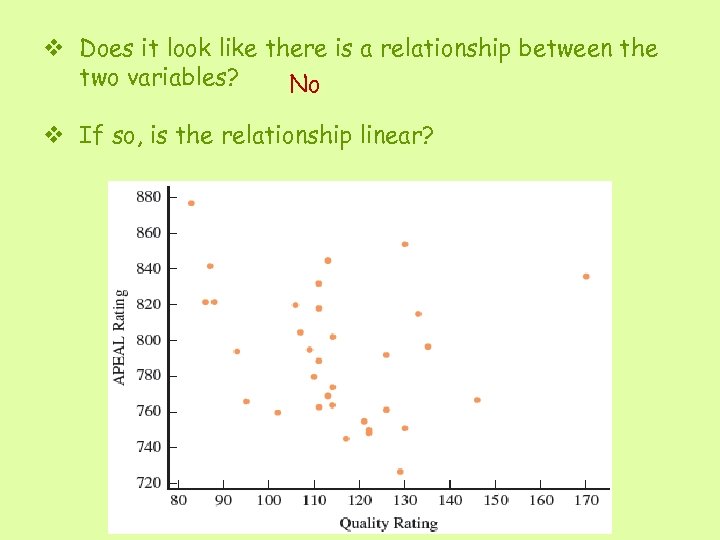
v Does it look like there is a relationship between the two variables? No v If so, is the relationship linear?
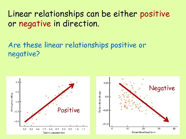
Linear relationships can be either positive or negative in direction. Are these linear relationships positive or negative? Negative Positive
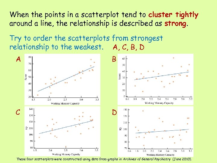
When the points in a scatterplot tend to cluster tightly around a line, the relationship is described as strong. Try to order the scatterplots from strongest relationship to the weakest. A, C, B, D A B C D These four scatterplots were constructed using data from graphs in Archives of General Psychiatry (June 2010).
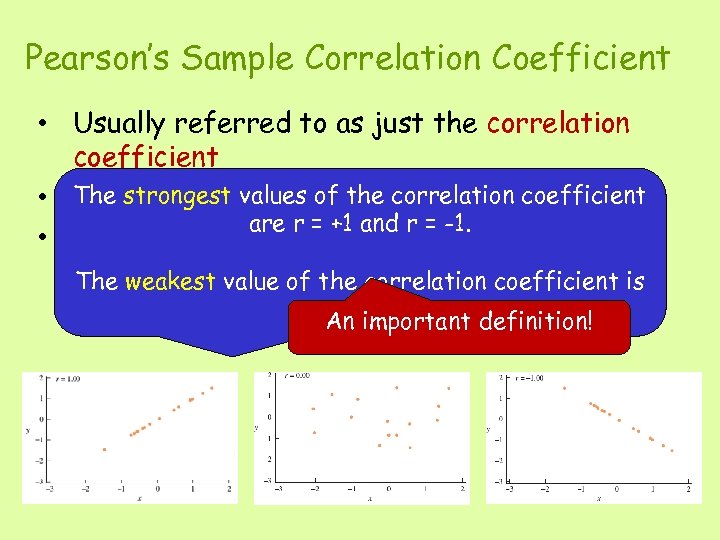
Pearson’s Sample Correlation Coefficient • Usually referred to as just the correlation coefficient • The strongestrvalues of the correlation coefficient Denoted by are r = +1 and r = -1. • Measures the strength and direction of a linear relationship between two numerical is The weakest value of the correlation coefficient variables r = 0. An important definition!
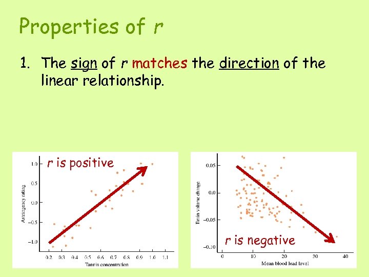
Properties of r 1. The sign of r matches the direction of the linear relationship. r is positive r is negative
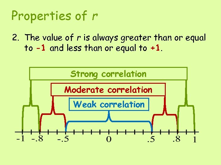
Properties of r 2. The value of r is always greater than or equal to -1 and less than or equal to +1. Strong correlation Moderate correlation Weak correlation
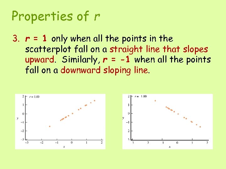
Properties of r 3. r = 1 only when all the points in the scatterplot fall on a straight line that slopes upward. Similarly, r = -1 when all the points fall on a downward sloping line.
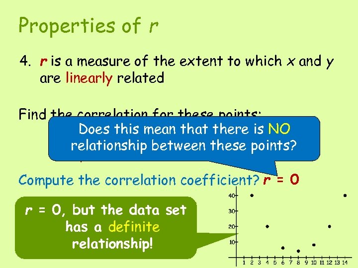
Properties of r 4. r is a measure of the extent to which x and y are linearly related Find the correlation for these points: Does this mean that there is NO x 2 4 6 8 10 12 14 relationship between these points? y 40 20 8 4 8 20 40 Compute the correlation coefficient? r = 0 Sketch the scatterplot. r = 0, but the data set has a definite relationship!
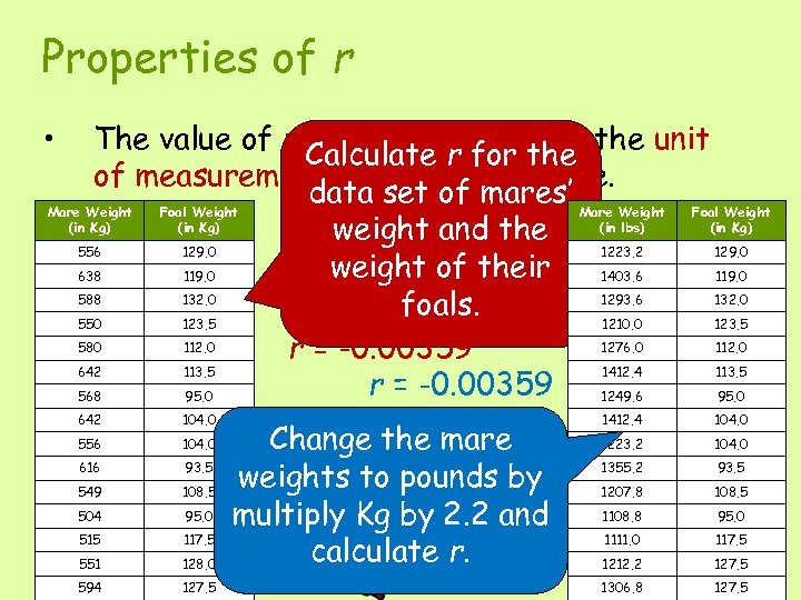
Properties of r • The value of r does not depend on the unit Calculate r for the of measurement for either variable. data set of mares’ Mare Weight Foal Weight (in Kg) (in lbs) (in Kg) weight and the 556 129. 0 1223. 2 129. 0 weight of their 638 119. 0 1403. 6 119. 0 588 132. 0 1293. 6 132. 0 foals. 550 123. 5 1210. 0 123. 5 580 112. 0 1276. 0 112. 0 r = -0. 00359 642 113. 5 1412. 4 113. 5 r = -0. 00359 568 95. 0 1249. 6 95. 0 642 104. 0 556 104. 0 616 93. 5 549 108. 5 504 95. 0 515 117. 5 551 128. 0 594 127. 5 Change the mare weights to pounds by multiply Kg by 2. 2 and calculate r. 1412. 4 104. 0 1223. 2 104. 0 1355. 2 93. 5 1207. 8 108. 5 1108. 8 95. 0 1111. 0 117. 5 1212. 2 127. 5 1306. 8 127. 5
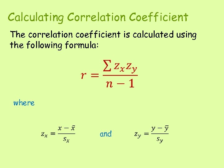
Calculating Correlation Coefficient The correlation coefficient is calculated using the following formula: where and
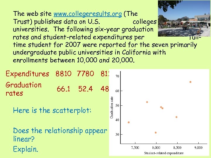
The web site www. collegeresults. org (The Education Trust) publishes data on U. S. colleges and universities. The following six-year graduation rates and student-related expenditures per fulltime student for 2007 were reported for the seven primarily undergraduate public universities in California with enrollments between 10, 000 and 20, 000. Expenditures 8810 7780 8112 8149 8477 7342 7984 Graduation rates 66. 1 52. 4 48. 9 Here is the scatterplot: Does the relationship appear linear? Explain. 48. 1 42. 0 38. 3 31. 3
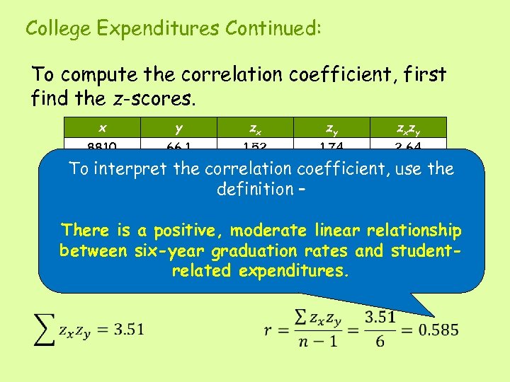
College Expenditures Continued: To compute the correlation coefficient, first find the z-scores. x y zx zy zxzy 8810 66. 1 1. 52 1. 74 2. 64 8149 48. 1 0. 12 0. 01 -0. 66 0. 51 To 7780 interpret 52. 4 correlation coefficient, -0. 34 the use 8112 48. 9 0. 04 0. 01 definition – 0. 19 8477 42. 0 0. 81 -0. 42 -0. 34 There is a positive, moderate linear relationship 7342 38. 3 -1. 59 -0. 76 1. 21 between six-year graduation rates and student 7984 31. 3 -0. 23 -1. 38 0. 32 related expenditures.
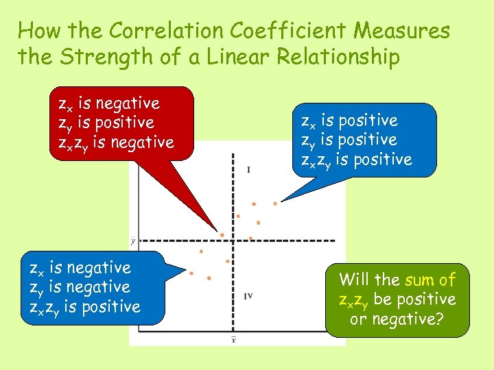
How the Correlation Coefficient Measures the Strength of a Linear Relationship zx is negative zy is positive zxzy is negative zx is negative zy is negative zxzy is positive zx is positive zy is positive zxzy is positive Will the sum of zxzy be positive or negative?
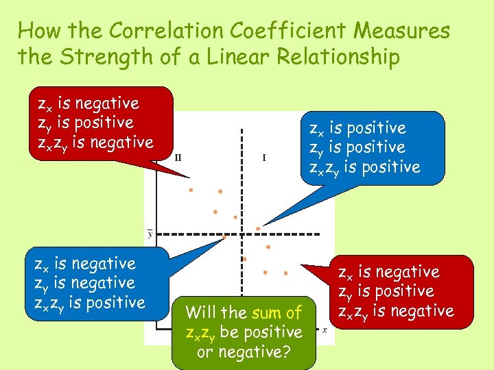
How the Correlation Coefficient Measures the Strength of a Linear Relationship zx is negative zy is positive zxzy is negative zx is negative zy is negative zxzy is positive zx is positive zy is positive zxzy is positive Will the sum of zxzy be positive or negative? zx is negative zy is positive zxzy is negative
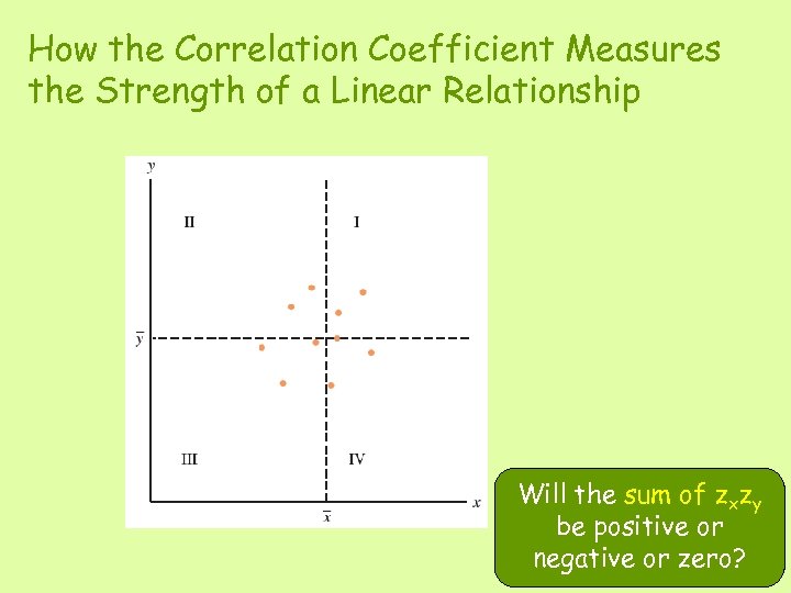
How the Correlation Coefficient Measures the Strength of a Linear Relationship Will the sum of zxzy be positive or negative or zero?
Does a value of r close to 1 or -1 mean that a change in one variable causes a change in the other variable? Association does NOT imply causation. Consider the following examples: • The relationship between the number of Causality child’s be hot cavities in aall drink more shown by carefully Should we can onlyteeth and the size of controllingare responses to cold weather positive. Both lower of all variables and chocolate tovocabulary is rate? his or her valuesthe crime strong that might be related to the ones under study. In other words, with amean I should feed children more So does this well-controlled, well-designed • Consumption to increase their vocabulary? These chocolate both strongly candy of hot variables areis negatively experiment. related rate. correlated with crimeto the age of the child
Linear Regression Least Squares Regression Line
Suppose there is a relationship between two numerical variables. Let x be the amount spent on advertising and y be the amount of sales for the product during a given period. The othe r variable , de product You predictor vato predict noted by sales (y) for a might want x, is the riable (so ind when the meti on month ependent amount spentmesadvertising is called or explan atory var $10, 000 (x). ieblariable a ed th v e). to denot d response r y is use The lette called the , o predict u want t variable). yo ependent d iable (or var
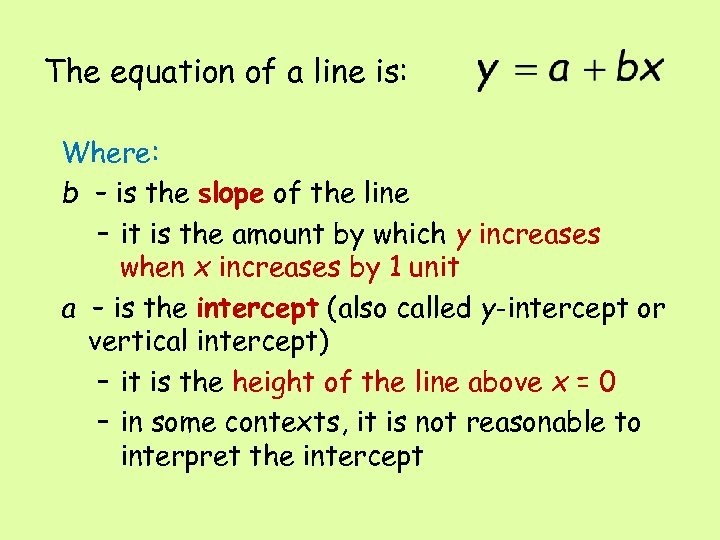
The equation of a line is: Where: b – is the slope of the line – it is the amount by which y increases when x increases by 1 unit a – is the intercept (also called y-intercept or vertical intercept) – it is the height of the line above x = 0 – in some contexts, it is not reasonable to interpret the intercept
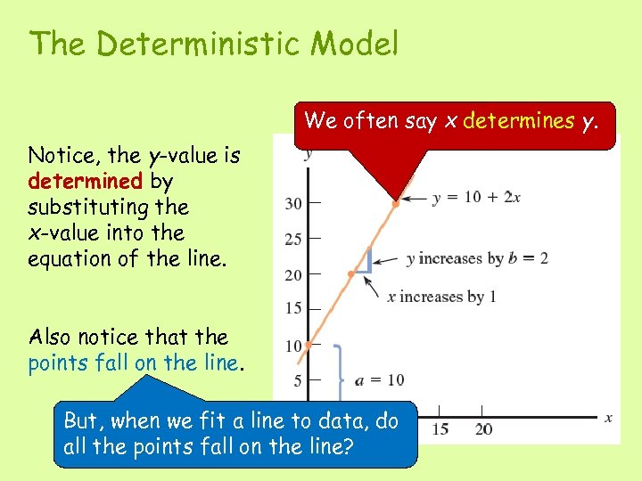
The Deterministic Model We often say x determines y. Notice, the y-value is determined by substituting the x-value into the equation of the line. Also notice that the points fall on the line. But, when we fit a line to data, do all the points fall on the line?
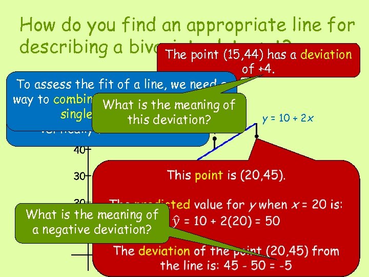
How do you find an appropriate line for describing a bivariate data set? a deviation The point (15, 44) has To assess the fit of a line, we need a way to combine What deviations into of To assess the of is line, meaning a fit n a the we look atsingle measure of fit. how the points deviate this deviation? vertically from the line. What is the meaning of a negative deviation? of +4. y = 10 + 2 x
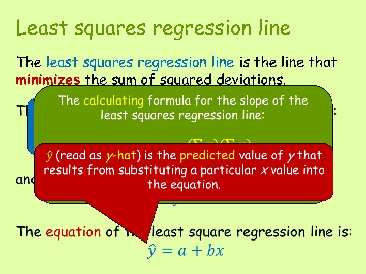
Least squares regression line The least squares regression line is the line that minimizes the sum of squared deviations. The most widely used measure of the fit of a line y = a + bx to bivariate data is the sum of the squared deviations about the line.
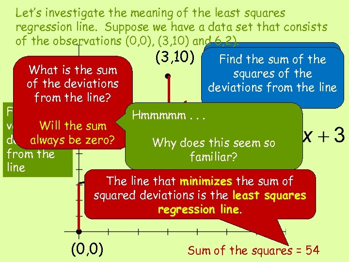
Let’s investigate the meaning of the least squares regression line. Suppose we have a data set that consists of the observations (0, 0), (3, 10) and 6, 2). Use the sum of the (3, 10) Find a calculator to findsquares of squares the least the What is the sum regression the of the deviations fromline from the line? 6. . . Find the Hmmmmm Will vertical the sum always deviations be zero? Why does this seem so from the familiar? line -3 The line that minimizes the sum of squared deviations is the least squares (6, 2) -3 regression line (0, 0) Sum of the squares = 54
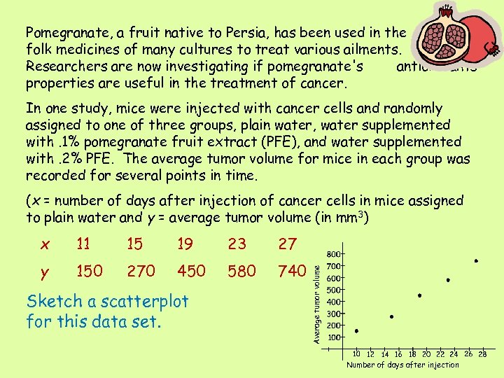
Pomegranate, a fruit native to Persia, has been used in the folk medicines of many cultures to treat various ailments. Researchers are now investigating if pomegranate's antioxidants properties are useful in the treatment of cancer. In one study, mice were injected with cancer cells and randomly assigned to one of three groups, plain water, water supplemented with. 1% pomegranate fruit extract (PFE), and water supplemented with. 2% PFE. The average tumor volume for mice in each group was recorded for several points in time. (x = number of days after injection of cancer cells in mice assigned to plain water and y = average tumor volume (in mm 3) 11 15 19 23 27 y 150 270 450 580 740 Sketch a scatterplot for this data set. Average tumor volume x Number of days after injection
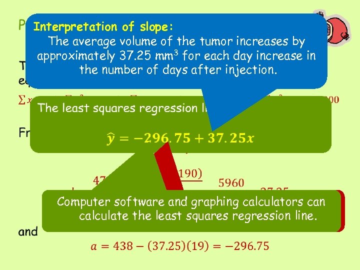
Interpretation of slope: The average volume of the tumor increases by approximately 37. 25 mm 3 for each day increase in the number of days after injection. Computer software and graphing calculators can Does the intercept have meaning in this calculate the least squares regression line. context? Why or why not?
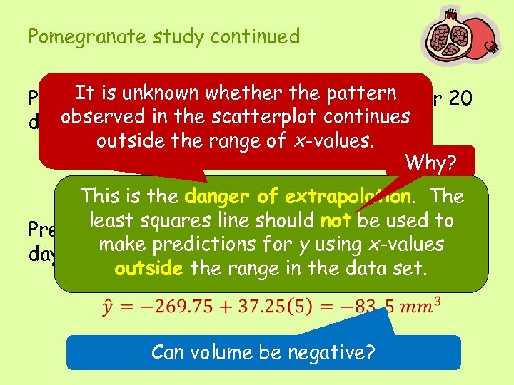
Pomegranate study continued It the average volume the pattern Predict is unknown whether of the tumor for 20 observed in the scatterplot continues days after injection. outside the range of x-values. Why? This is the danger of extrapolation. The least squares volume of not be used to Predict the average line shouldthe tumor for 5 make predictions for y using x-values days after injection. outside the range in the data set. Can volume be negative?
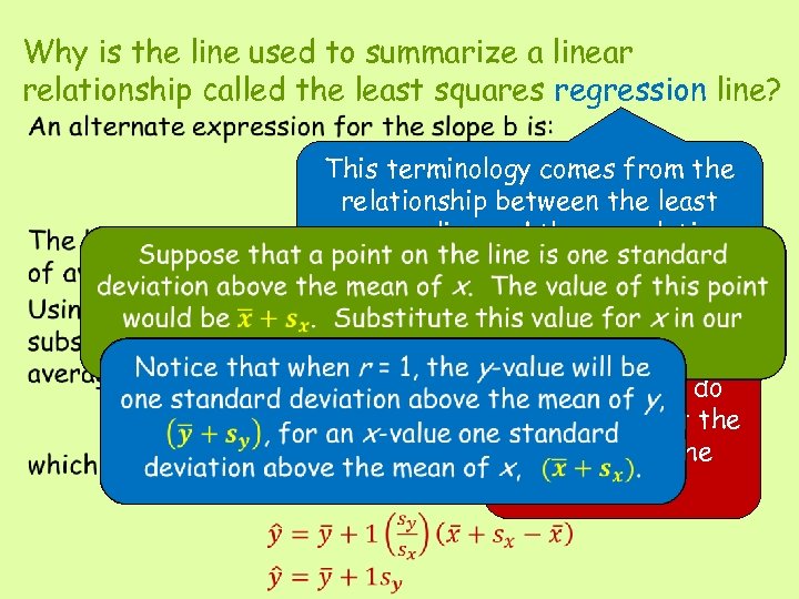
Why is the line used to summarize a linear relationship called the least squares regression line? • This terminology comes from the relationship between the least squares line and the correlation coefficient. If r = 1, what do you know about the location of the points?
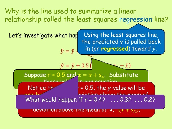
Why is the line used to summarize a linear relationship called the least squares regression line? What would happen if r = 0. 4? . . . 0. 3? . . . 0. 2?
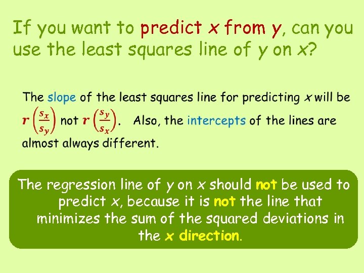
If you want to predict x from y, can you use the least squares line of y on x? The regression line of y on x should not be used to predict x, because it is not the line that minimizes the sum of the squared deviations in the x direction.
Assessing the Fit of a Line Residuals Residual Plots Outliers and Influential Points Coefficient of Determination Standard Deviation about the Line
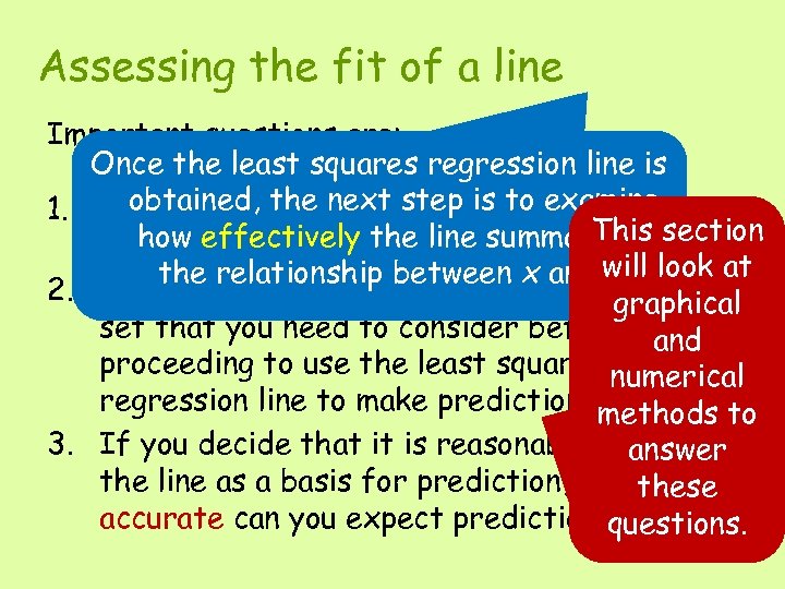
Assessing the fit of a line Important questions are: Once the least squares regression line is 1. Isobtained, an appropriate way to summarize the line the next step is to examine This how effectively the line summarizes section the relationship between x and y ? the relationship between x and will look at y. 2. Are there any unusual aspects of the data graphical set that you need to consider before and proceeding to use the least squares numerical regression line to make predictions? methods to 3. If you decide that it is reasonable toanswer use the line as a basis for prediction, how these accurate can you expect predictionsquestions. to be?
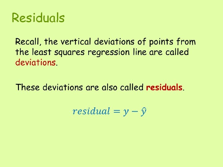
Residuals •
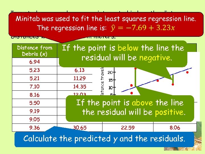
In a study, researchers were interested in how the distance a deer mouse will travel for food (y) is related to the distance from the food to the nearest pile of fine woody debris (x). Distances were measured in meters. 6. 94 If. Distance the point is below the line the Traveled (y) residual will be negative. 0. 00 14. 76 -14. 76 5. 23 6. 13 5. 21 11. 29 7. 10 14. 35 8. 16 12. 03 5. 50 9. 19 Distance traveled Distance from Debris (x) 22. 72 the If 9. 23 -3. 10 9. 16 2. 13 15. 28 -0. 93 18. 70 -6. 67 point 10. 10 is above the 12. 62 line 20. 11 22. 04 the residual Distance to debris -1. 93 will be positive. 9. 05 26. 16 21. 58 4. 58 9. 36 30. 65 22. 59 8. 06 Calculate the predicted y and the residuals.
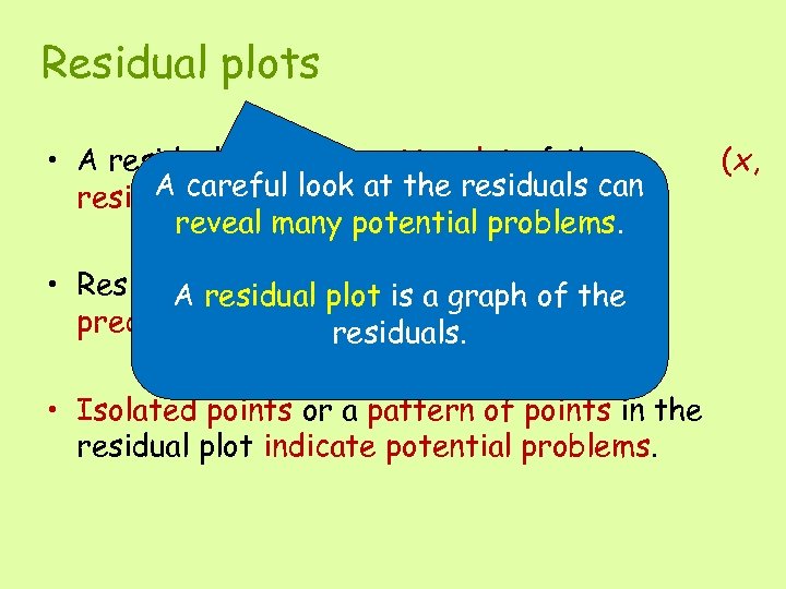
Residual plots • A residual plot is a scatterplot of the A careful residual) pairs. look at the residuals can reveal many potential problems. • Residualsresidual plot graphed against the A can also be is a graph of the predicted y-values residuals. • Isolated points or a pattern of points in the residual plot indicate potential problems. (x,
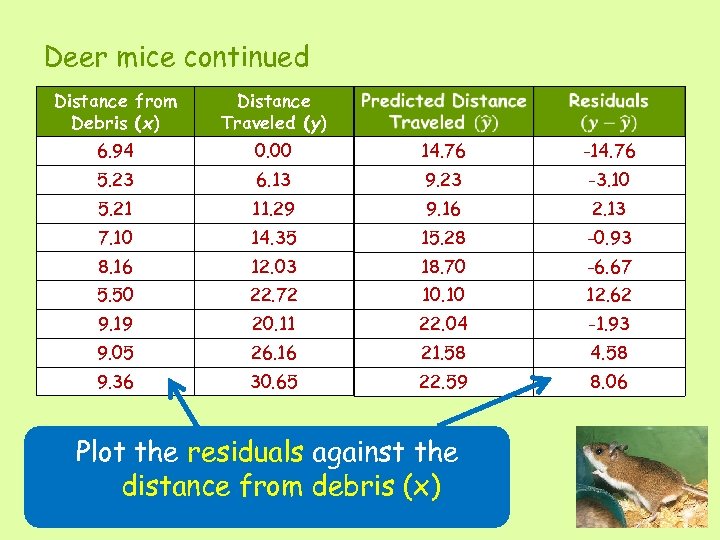
Deer mice continued Distance from Debris (x) Distance Traveled (y) 6. 94 0. 00 14. 76 -14. 76 5. 23 6. 13 9. 23 -3. 10 5. 21 11. 29 9. 16 2. 13 7. 10 14. 35 15. 28 -0. 93 8. 16 12. 03 18. 70 -6. 67 5. 50 22. 72 10. 10 12. 62 9. 19 20. 11 22. 04 -1. 93 9. 05 26. 16 21. 58 4. 58 9. 36 30. 65 22. 59 8. 06 Plot the residuals against the distance from debris (x)
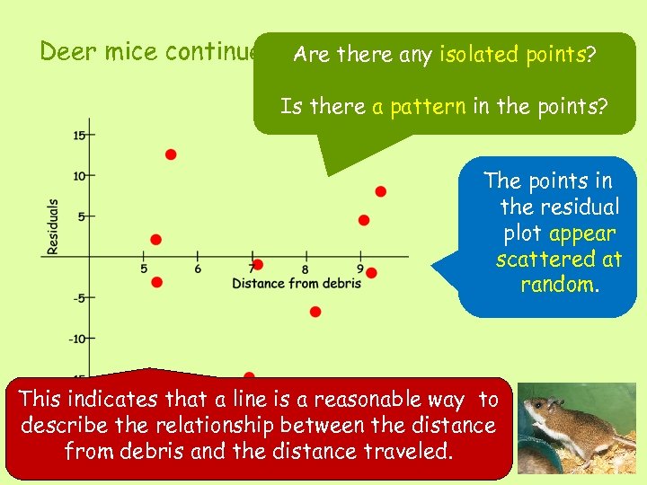
Deer mice continued Are there any isolated points? Is there a pattern in the points? The points in the residual plot appear scattered at random. This indicates that a line is a reasonable way to describe the relationship between the distance from debris and the distance traveled.
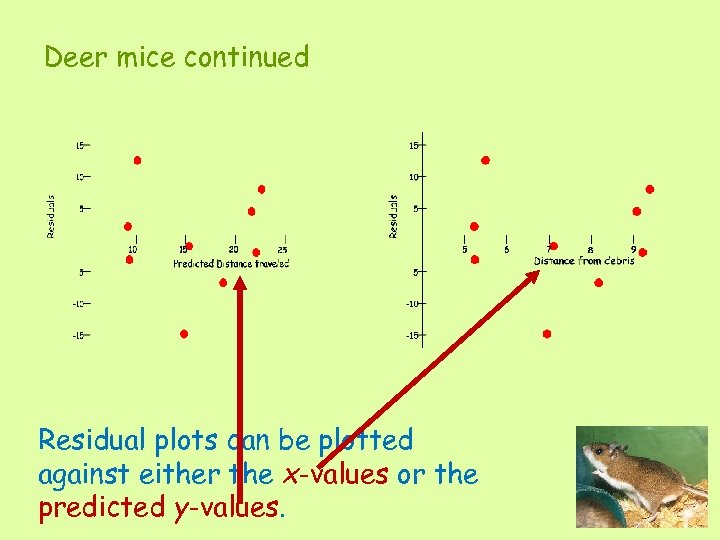
Deer mice continued Residual plots can be plotted against either the x-values or the predicted y-values.
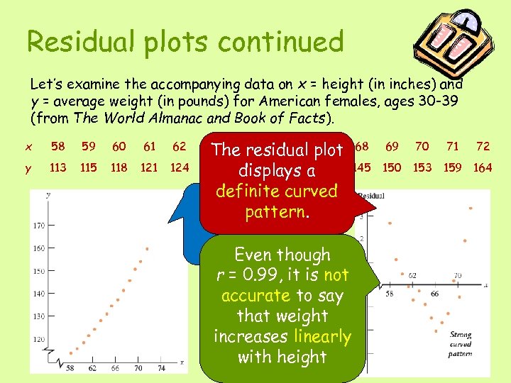
Residual plots continued Let’s examine the accompanying data on x = height (in inches) and y = average weight (in pounds) for American females, ages 30 -39 (from The World Almanac and Book of Facts). x 58 59 60 61 62 y 113 115 118 121 124 63 64 residual The 65 66 67 plot 68 128 131 134 137 141 145 displays a definite curved The scatterplot pattern. appears rather straight. Even though r = 0. 99, it is not accurate to say that weight increases linearly with height 69 70 71 72 150 153 159 164
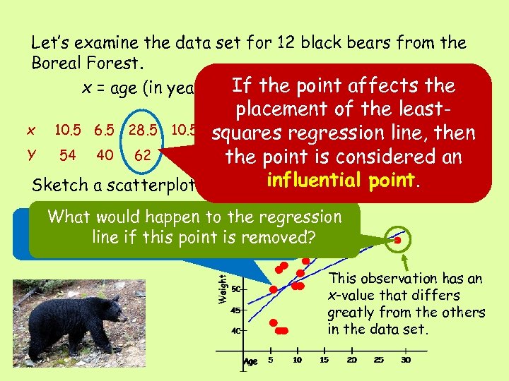
Let’s examine the data set for 12 black bears from the Boreal Forest. If the point affects the x = age (in years) and y = weight (in kg) placement of the leastx 10. 5 6. 5 28. 5 10. 5 6. 5 7. 5 6. 5 5. 5 7. 5 11. 5 9. 5 5. 5 squares regression line, then Y 54 40 62 51 55 56 62 is considered an 50 the point 42 40 59 51 Sketch a scatterplot with theinfluential point. fitted regression line. What would anything the regression Do you notice happen tounusual line if this point is removed? about this data set? This observation has an x-value that differs greatly from the others in the data set.
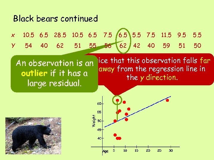
Black bears continued x Y 10. 5 6. 5 28. 5 10. 5 6. 5 54 40 62 51 55 7. 5 6. 5 5. 5 7. 5 11. 5 9. 5 56 62 50 42 40 59 51 Notice that this observation falls far An observation is an away from the regression line in outlier if it has a the y direction. large residual.
Coefficient of Determination • The coefficient of determination is the Suppose that proportion ofyou would like to predict the price of variation in y that can be houses in a particular city from the size of the house attributedfeet). There will be variability in house (in square to an approximate linear relationship is this variability that makes accurate price, and it between x & y price prediction a challenge. • Denoted by r 2 If you know that differences in house size account for a large proportion of the variability in house price, • The value of r 2 size of a house will help you predict then knowing the is often converted to a its price. percentage.
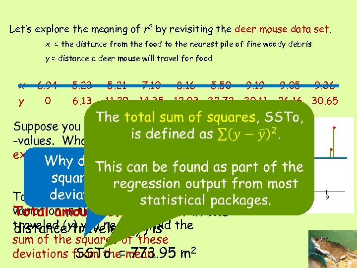
Let’s explore the meaning of r 2 by revisiting the deer mouse data set. x = the distance from the food to the nearest pile of fine woody debris y = distance a deer mouse will travel for food x 6. 94 5. 23 5. 21 y 0 6. 13 11. 29 7. 10 8. 16 5. 50 9. 19 14. 35 12. 03 22. 72 20. 11 Suppose you didn’t know any x -values. What distance would you expect deer mice to travel? Why do we square the deviations? To find the total amount of variation in the distance Total amount of variation in the traveled (y) you need (y) find the distance traveled to is sum of the squares of these deviations from the mean. SSTo = 773. 95 m 2 9. 05 9. 36 26. 16 30. 65
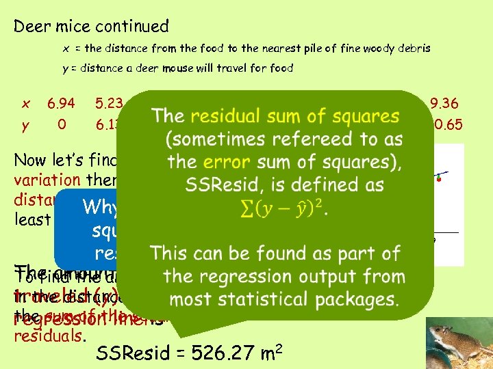
Deer mice continued x = the distance from the food to the nearest pile of fine woody debris y = distance a deer mouse will travel for food 6. 94 5. 23 y 0 6. 13 5. 21 11. 29 7. 10 8. 16 5. 50 9. 19 14. 35 12. 03 22. 72 20. 11 Now let’s find how much variation there is in the distance traveled (y) from the Why do we least squares regression line. Distance traveled x 9. 05 26. 16 30. 65 square the Distance to debris residuals? The amount of variation in the distance To find the amount of variation in the distance traveled least traveled (y) from the(y), findsquares the sum of the squared regression line is residuals. SSResid = 526. 27 m 2 9. 36
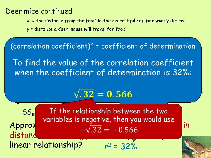
Deer mice continued x = the distance from the food to the nearest pile of fine woody debris y = distance a deer mouse will travel for food Total amount of variation in the distance traveled (y) is SSTO = 773. 95 m 2. The amount of variation in y values from the regression line is How does the variation in y change when we used the least squares regression line? SSResid = 526. 27 m 2 Approximately what percent of the variation in distance traveled (y) can be explained by the linear relationship? r 2 = 32%
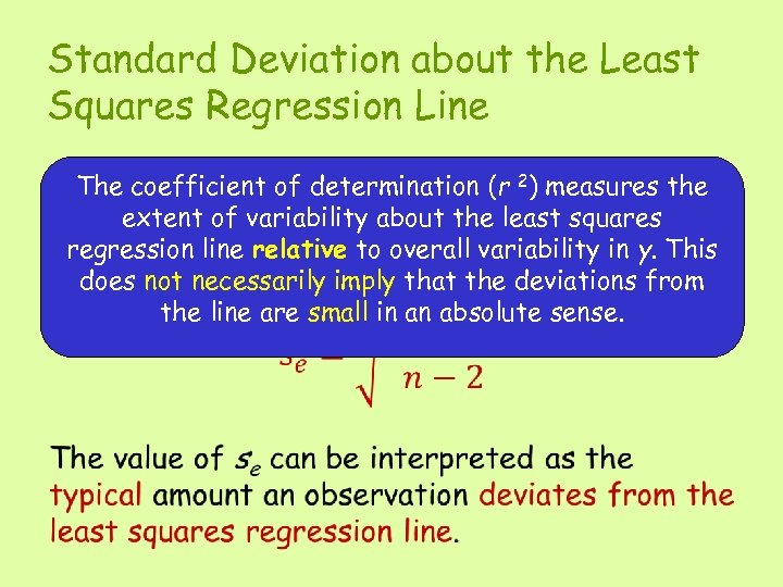
Standard Deviation about the Least Squares Regression Line • The coefficient of determination (r 2) measures the extent of variability about the least squares regression line relative to overall variability in y. This does not necessarily imply that the deviations from the line are small in an absolute sense.
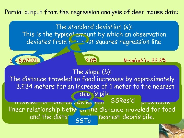
Partial output from the regression analysis of deer mouse data: The standard deviation (s): Predictor T P This is the typical. Coef amount SE Coef an observation by which Constant -7. 69 13. 33 -0. 582 deviates from the least squares regression line Distance to debris S = 8. 67071 3. 234 R-sq = 32. 0% 1. 782 1. 82 0. 112 R-sq(adj) = 22. 3% The y-intercept (a): The slope (b): Analysis of Variance This value has no meaning in context since it doesn't The distance traveled to food increases by approximately P Source DF SS MS F make sense to have a negative distance. 3. 234 meters for an 247. 68 determination to 3. 29 nearest increase of 1 meter (r 2 the The coefficient of ): Regression 1 247. 68 0. 112 debris pile. Only 32% of the observed variability in the distance Resid Error 7 526. 27 75. 18 SSResid traveled for food can 773. 95 be explained by the approximate Total 8 linear relationship between the distance traveled for food and the distance to the nearest debris pile. SSTo
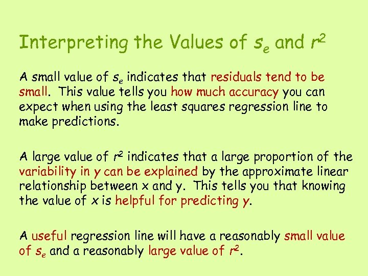
Interpreting the Values of se and r 2 A small value of se indicates that residuals tend to be small. This value tells you how much accuracy you can expect when using the least squares regression line to make predictions. A large value of r 2 indicates that a large proportion of the variability in y can be explained by the approximate linear relationship between x and y. This tells you that knowing the value of x is helpful for predicting y. A useful regression line will have a reasonably small value of se and a reasonably large value of r 2.
![A study (Archives of General Psychiatry[2010]: 570 -577) looked at how working memory typical A study (Archives of General Psychiatry[2010]: 570 -577) looked at how working memory typical](https://present5.com/presentation/04e4a65dd8d1b0f378258d785eafe35c/image-55.jpg)
A study (Archives of General Psychiatry[2010]: 570 -577) looked at how working memory typical deviation of the For the patient group, the capacity was related to For the control group, the typical deviation of the scores on a test ofthe regression line is about 10. 7, which observations from cognitive functioning and to scores on observations from the regression line is about 6. 1, which is an somewhat Two groups were studied – (a relatively small is IQ test. large. Approximately 14% one group smaller. Approximately 79% (a much larger amount) of the consisted of patients diagnosed with schizophrenia and amount) of the variation in the cognitive functioning score is explained by the otheris explained by the linear relationship. group consisted of healthy control subjects. the regression line. Thus, the regression line for the control group would produce more accurate predictions than the regression line for the patient group.

Putting it All Together Describing Linear Relationships Making Predictions
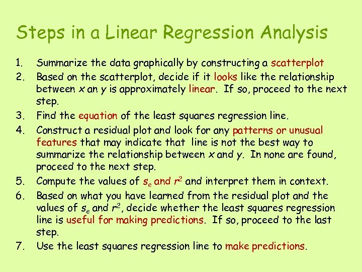
Steps in a Linear Regression Analysis 1. 2. 3. 4. 5. 6. 7. Summarize the data graphically by constructing a scatterplot Based on the scatterplot, decide if it looks like the relationship between x an y is approximately linear. If so, proceed to the next step. Find the equation of the least squares regression line. Construct a residual plot and look for any patterns or unusual features that may indicate that line is not the best way to summarize the relationship between x and y. In none are found, proceed to the next step. Compute the values of se and r 2 and interpret them in context. Based on what you have learned from the residual plot and the values of se and r 2, decide whether the least squares regression line is useful for making predictions. If so, proceed to the last step. Use the least squares regression line to make predictions.
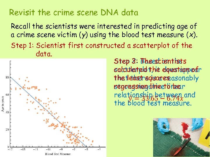
Revisit the crime scene DNA data Recall the scientists were interested in predicting age of a crime scene victim (y) using the blood test measure (x). Step 1: Scientist first constructed a scatterplot of the data. Step 2: Based on the scatterplot, it does appear that there is a reasonably strong negative linear relationship between and the blood test measure.
Step 4: A residual plot constructed from these data showed a few observations with large residuals, but these observations were not far removed from the rest of the data in the x direction. The observations were not judged to be influential. Also there were no unusual patterns in the residual plot that would suggest a nonlinear relationship between age and the blood test measure. Step 5: se = 8. 9 and r 2 = 0. 835 Approximately 83. 5% of the variability in age can be explained by the linear relationship. A typical difference between the predicted age and the actual age would be about 9 years.
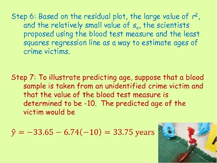
Step 6: Based on the residual plot, the large value of r 2, and the relatively small value of se, the scientists proposed using the blood test measure and the least squares regression line as a way to estimate ages of crime victims.
Modeling Nonlinear Relationships
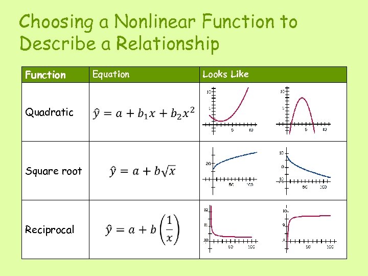
Choosing a Nonlinear Function to Describe a Relationship Function Equation Quadratic Square root Reciprocal Looks Like
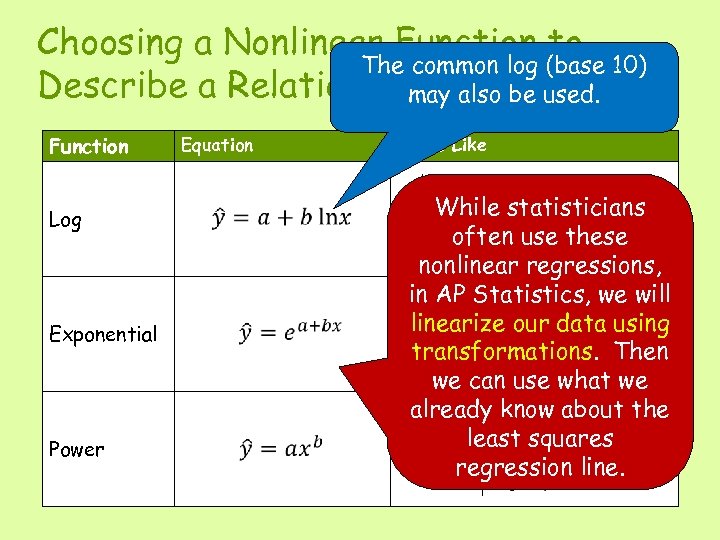
Choosing a Nonlinear Function to The common log (base 10) Describe a Relationship also be used. may Function Log Equation Exponential Power Looks Like While statisticians often use these nonlinear regressions, in AP Statistics, we will linearize our data using transformations. Then we can use what we already know about the least squares regression line.
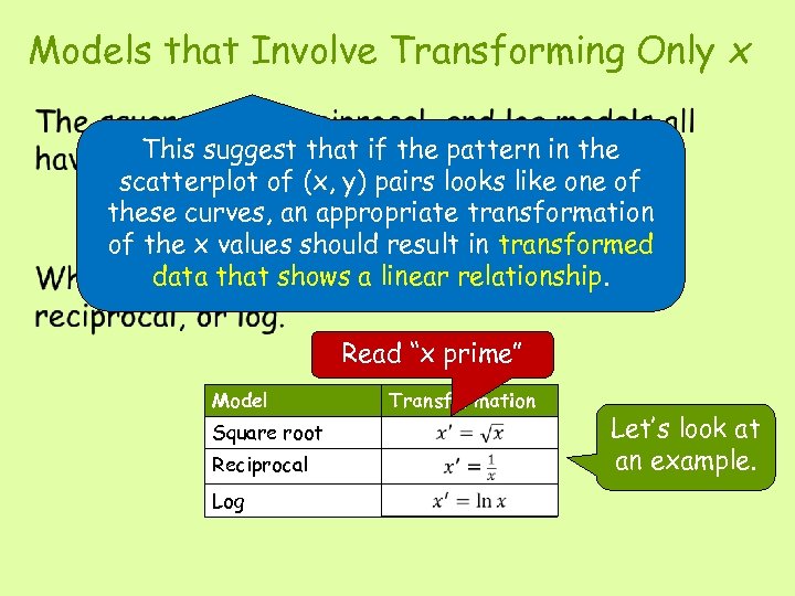
Models that Involve Transforming Only x • This suggest that if the pattern in the scatterplot of (x, y) pairs looks like one of these curves, an appropriate transformation of the x values should result in transformed data that shows a linear relationship. Read “x prime” Model Square root Reciprocal Log Transformation Let’s look at an example.
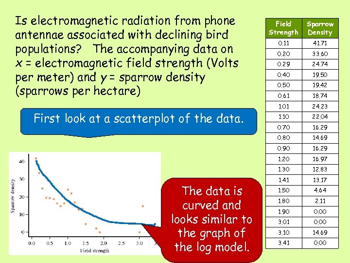
Is electromagnetic radiation from phone antennae associated with declining bird populations? The accompanying data on x = electromagnetic field strength (Volts per meter) and y = sparrow density (sparrows per hectare) 0. 11 41. 71 0. 20 33. 60 0. 29 24. 74 0. 40 19. 50 0. 50 19. 42 0. 61 18. 74 1. 01 24. 23 1. 10 22. 04 0. 70 16. 29 14. 69 0. 90 16. 29 1. 20 16. 97 1. 30 The data is curved and looks similar to the graph of the log model. Sparrow Density 0. 80 First look at a scatterplot of the data. Field Strength 12. 83 1. 41 13. 17 1. 50 4. 64 1. 80 2. 11 1. 90 0. 00 3. 01 0. 00 3. 10 14. 69 3. 41 0. 00
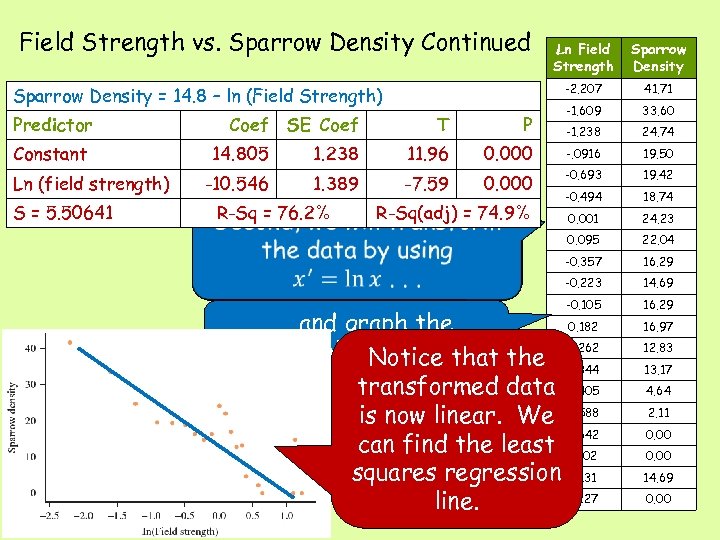
Field Strength vs. Sparrow Density Continued Predictor Sparrow Density -2. 207 Sparrow Density = 14. 8 – ln (Field Strength) Ln Field Strength 41. 71 -1. 609 33. 60 -1. 238 24. 74 Coef SE Coef T P 14. 805 1. 238 11. 96 0. 000 -. 0916 19. 50 Ln (field strength) -10. 546 1. 389 -7. 59 0. 000 -0. 693 19. 42 S = 5. 50641 R-Sq = 76. 2% -0. 494 18. 74 0. 001 24. 23 0. 095 22. 04 -0. 357 16. 29 -0. 223 14. 69 -0. 105 16. 29 Constant R-Sq(adj) = 74. 9% 0. 182. . . and graph the scatterplot Notice that the 0. 262 of y on x’ 0. 344 transformed data 0. 405 is now linear. We 0. 588 0. 642 can find the least 1. 102 squares regression 1. 131 1. 227 line. 16. 97 12. 83 13. 17 4. 64 2. 11 0. 00 14. 69 0. 00
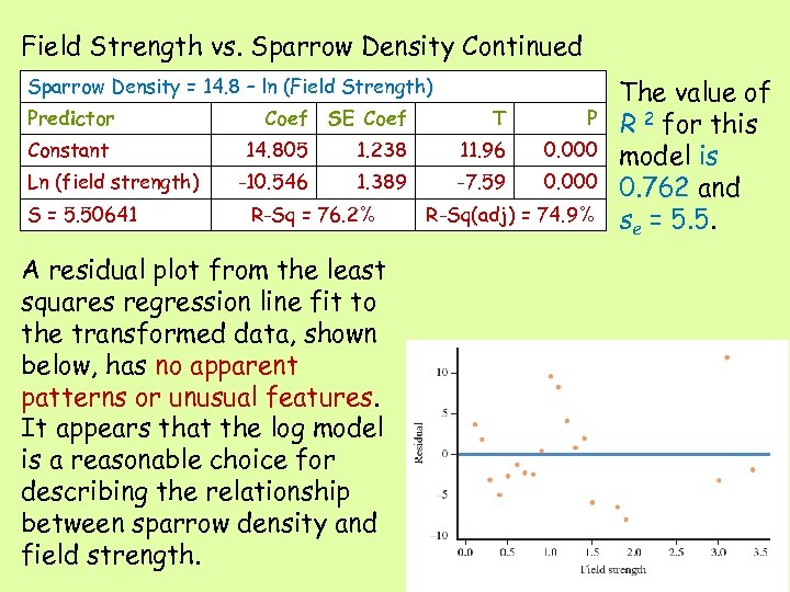
Field Strength vs. Sparrow Density Continued Sparrow Density = 14. 8 – ln (Field Strength) Predictor Constant Ln (field strength) S = 5. 50641 Coef SE Coef T P 14. 805 1. 238 11. 96 0. 000 -10. 546 1. 389 -7. 59 0. 000 R-Sq = 76. 2% A residual plot from the least squares regression line fit to the transformed data, shown below, has no apparent patterns or unusual features. It appears that the log model is a reasonable choice for describing the relationship between sparrow density and field strength. R-Sq(adj) = 74. 9% The value of R 2 for this model is 0. 762 and se = 5. 5.
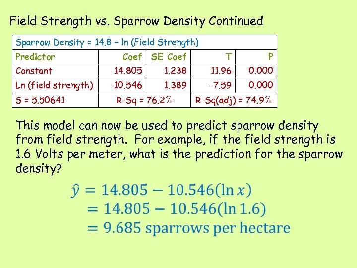
Field Strength vs. Sparrow Density Continued Sparrow Density = 14. 8 – ln (Field Strength) Predictor Coef Ln (field strength) S = 5. 50641 T P 14. 805 Constant SE Coef 1. 238 11. 96 0. 000 -10. 546 1. 389 -7. 59 0. 000 R-Sq = 76. 2% R-Sq(adj) = 74. 9% This model can now be used to predict sparrow density from field strength. For example, if the field strength is 1. 6 Volts per meter, what is the prediction for the sparrow density?
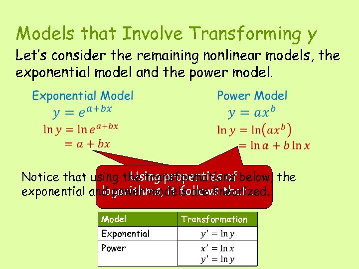
Models that Involve Transforming y Let’s consider the remaining nonlinear models, the exponential model and the power model. Using properties of Notice that using the transformations below, the logarithms, it follows that. . . exponential and power models are linearized. Model Exponential Power Transformation
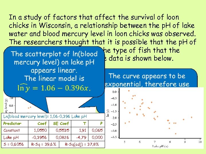
In a study of factors that affect the survival of loon chicks in Wisconsin, a relationship between the p. H of lake water and blood mercury level in loon chicks was observed. The researchers thought that it is possible that the p. H of the lake could be related to the type of fish that the loons ate. A scatterplot of the data is shown below. Ln(blood mercury level)= 1. 06 -0. 396 Lake p. H Predictor Coef SE Coef T P Constant 1. 0550 0. 5535 1. 91 0. 065 Lake p. H -0. 3956 0. 0826 -4. 79 0. 000 S = 0. 6056 R-Sq = 39. 6% R-Sq(adj) = 37. 8%
Choosing Among Different Possible Nonlinear Models Often there is more than one reasonable model that could be used to describe a nonlinear relationship between two variables. How do you choose a model? 1) Consider scientific theory. Does it suggest what model the relationship is? 2) In the absence of scientific theory, choose a model that has small residuals (small se) and accounts for a large proportion of the variability in y (large R 2).
Common Mistakes
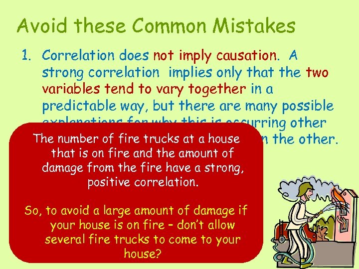
Avoid these Common Mistakes 1. Correlation does not imply causation. A strong correlation implies only that the two variables tend to vary together in a predictable way, but there are many possible explanations for why this is occurring other The number variable causing house in the other. than one of fire trucks at a change that is on fire and the amount of damage from the fire have a strong, Don’t fall into this trap! positive correlation. So, to avoid a large amount of damage if your house is on fire – don’t allow several fire trucks to come to your house?
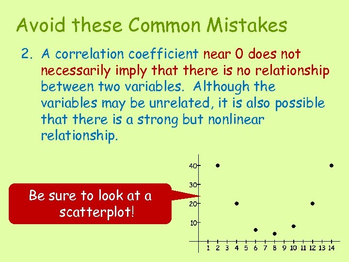
Avoid these Common Mistakes 2. A correlation coefficient near 0 does not necessarily imply that there is no relationship between two variables. Although the variables may be unrelated, it is also possible that there is a strong but nonlinear relationship. Be sure to look at a scatterplot!
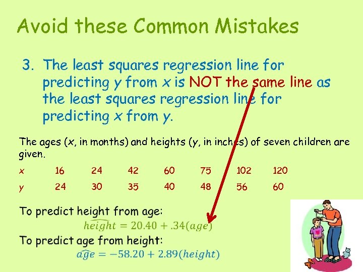
Avoid these Common Mistakes 3. The least squares regression line for predicting y from x is NOT the same line as the least squares regression line for predicting x from y. The ages (x, in months) and heights (y, in inches) of seven children are given. x 16 24 42 60 75 102 120 y 24 30 35 40 48 56 60
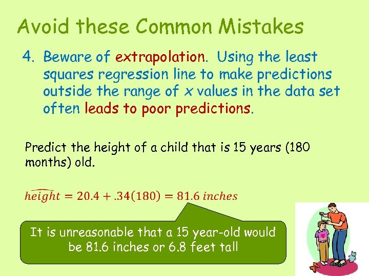
Avoid these Common Mistakes 4. Beware of extrapolation. Using the least squares regression line to make predictions outside the range of x values in the data set often leads to poor predictions. Predict the height of a child that is 15 years (180 months) old. It is unreasonable that a 15 year-old would be 81. 6 inches or 6. 8 feet tall
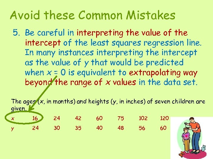
Avoid these Common Mistakes 5. Be careful in interpreting the value of the intercept of the least squares regression line. In many instances interpreting the intercept as the value of y that would be predicted when x = 0 is equivalent to extrapolating way beyond the range of x values in the data set. The ages (x, in months) and heights (y, in inches) of seven children are given. x 16 24 42 60 75 102 120 y 24 30 35 40 48 56 60
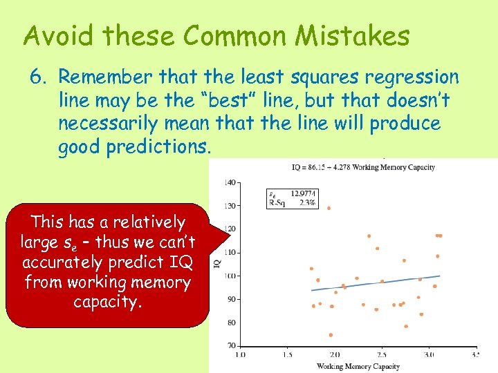
Avoid these Common Mistakes 6. Remember that the least squares regression line may be the “best” line, but that doesn’t necessarily mean that the line will produce good predictions. This has a relatively large se – thus we can’t accurately predict IQ from working memory capacity.
Avoid these Common Mistakes 7. It is not enough to look at just r 2 or just se when evaluating the regression line. Remember to consider both values. In general, your would like to have both a small value for se and a large value for r 2. This indicates that deviations from This indicates that the linear the line tend to be small. relationship explains a large proportion of the variability in the y values.
Avoid these Common Mistakes 8. The value of the correlation coefficient, as well as the values for the intercept and slope of the least squares regression line, can be sensitive to influential observations in the data set, particularly if the sample size is small. Be sure to always start with a plot to check for potential influential observations.
04e4a65dd8d1b0f378258d785eafe35c.ppt