Chapter 3 Uncertainty variation arises in data generated

Chapter 3: Uncertainty "variation arises in data generated by a model" "how to transform knowledge of this variation into statements about the uncertainty surrounding the model parameters" Confidence intervals via the frequentist/repeated sampling/classical approach

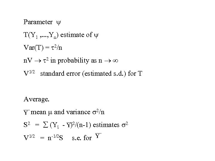Parameter T(Y 1 , . . . , Yn) estimate of Var(T) = 2/n n. V 2 in probability as n V 1/2 standard error (estimated s. d. ) for T Average. mean and variance 2/n S 2 = (Yi - )2/(n-1) estimates 2 V 1/2 = n-1/2 S s. e. for

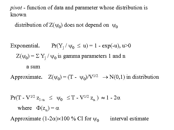pivot - function of data and parameter whose distribution is known distribution of Z( 0) does not depend on 0 Exponential. Pr(Yj / 0 u) = 1 - exp(-u), u>0 Z( 0) = Yj / 0 is gamma parameters 1 and n a sum Approximate. Z( 0) = (T - 0)/V 1/2 N(0, 1) in distribution Pr(T - V 1/2 z 1 - 0 T - V 1/2 z ) 1 - 2 where (z ) = Approximate (1 -2 ) 100 % CI for 0 interval estimate

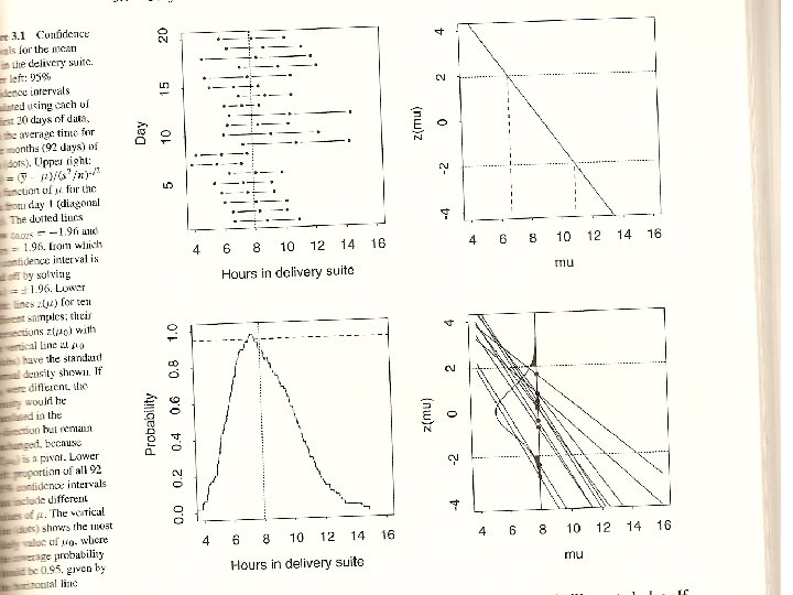
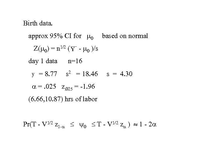Birth data. approx 95% CI for 0 Z( 0) = n 1/2 ( day 1 data = 8. 77 based on normal - 0 )/s n=16 s 2 = 18. 46 s = 4. 30 =. 025 z. 025 = -1. 96 (6. 66, 10. 87) hrs of labor Pr(T - V 1/2 z 1 - 0 T - V 1/2 z ) 1 - 2

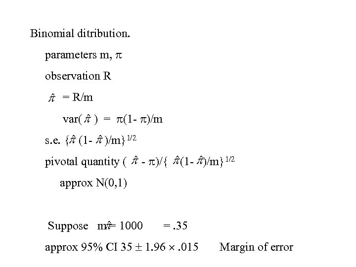Binomial ditribution. parameters m, observation R = R/m var( s. e. { (1 - ) = (1 - )/m}1/2 pivotal quantity ( - )/{ (1 - )/m}1/2 approx N(0, 1) Suppose m = 1000 =. 35 approx 95% CI 35 1. 96 . 015 Margin of error

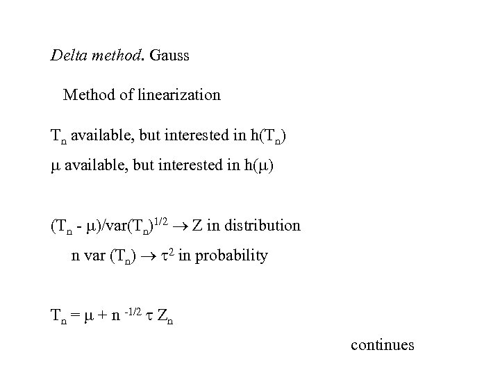Delta method. Gauss Method of linearization Tn available, but interested in h(Tn) available, but interested in h( ) (Tn - )/var(Tn)1/2 Z in distribution n var (Tn) 2 in probability Tn = + n -1/2 Zn continues

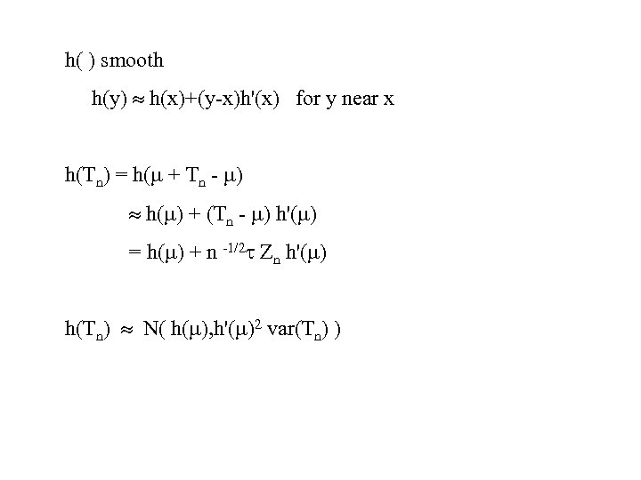h( ) smooth h(y) h(x)+(y-x)h'(x) for y near x h(Tn) = h( + Tn - ) h( ) + (Tn - ) h'( ) = h( ) + n -1/2 Zn h'( ) h(Tn) N( h( ), h'( )2 var(Tn) )

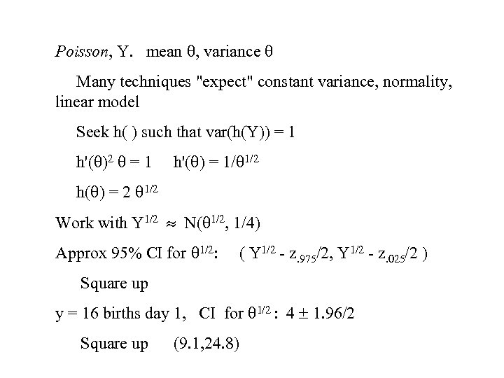Poisson, Y. mean , variance Many techniques "expect" constant variance, normality, linear model Seek h( ) such that var(h(Y)) = 1 h'( )2 = 1 h'( ) = 1/ 1/2 h( ) = 2 1/2 Work with Y 1/2 N( 1/2, 1/4) Approx 95% CI for 1/2: ( Y 1/2 - z. 975/2, Y 1/2 - z. 025/2 ) Square up y = 16 births day 1, CI for 1/2 : 4 1. 96/2 Square up (9. 1, 24. 8)

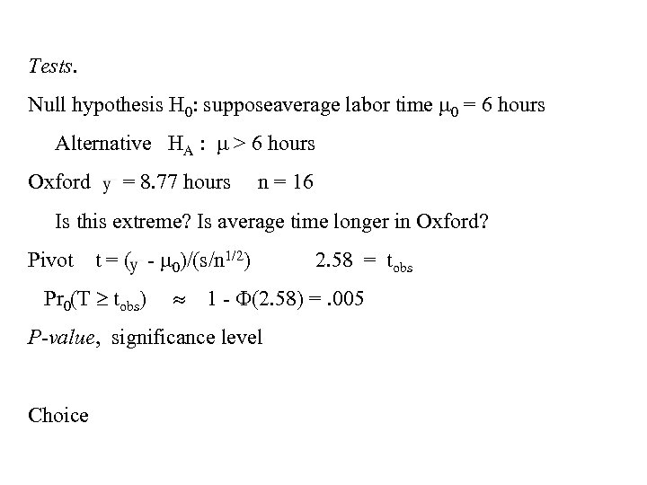Tests. Null hypothesis H 0: supposeaverage labor time 0 = 6 hours Alternative HA : > 6 hours Oxford = 8. 77 hours n = 16 Is this extreme? Is average time longer in Oxford? Pivot t = ( - 0)/(s/n 1/2) Pr 0(T tobs) 1 - (2. 58) =. 005 P-value, significance level Choice 2. 58 = tobs

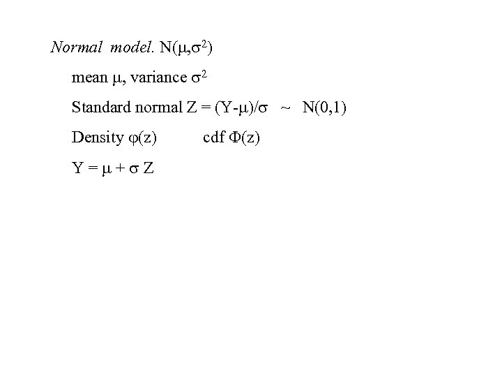Normal model. N( , 2) mean , variance 2 Standard normal Z = (Y- )/ ~ N(0, 1) Density (z) Y= + Z cdf (z)

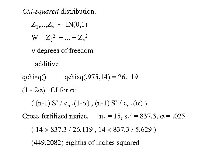Chi-squared distribution. Z 1, . . . , Z ~ IN(0, 1) W = Z 12 +. . . + Z 2 degrees of freedom additive qchisq() qchisq(. 975, 14) = 26. 119 (1 - 2 ) CI for 2 ( (n-1) S 2 / cn-1(1 - ) , (n-1) S 2 / cn-1( ) ) Cross-fertilized maize. n 1 = 15, s 12 = 837. 3, =. 025 ( 14 837. 3 / 26. 119 , 14 837. 3 / 5. 629 ) (449, 2082) eighths of inches squared

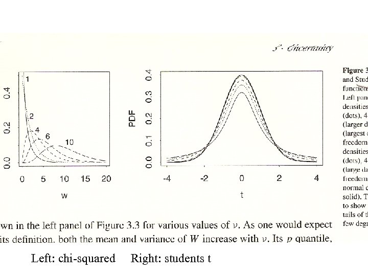Left: chi-squared Right: students t

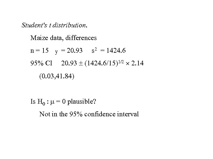Student's t distribution. Maize data, differences n = 15 = 20. 93 s 2 = 1424. 6 95% CI 20. 93 (1424. 6/15)1/2 2. 14 (0. 03, 41. 84) Is H 0 : = 0 plausible? Not in the 95% confidence interval

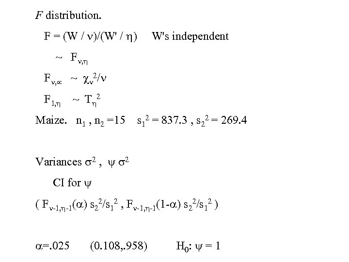F distribution. F = (W / )/(W' / ) W's independent ~ F , ~ 2/ F 1, ~ T 2 Maize. n 1 , n 2 =15 s 12 = 837. 3 , s 22 = 269. 4 Variances 2 , 2 CI for ( F -1, -1( ) s 22/s 12 , F -1, -1(1 - ) s 22/s 12 ) =. 025 (0. 108, . 958) H 0: = 1

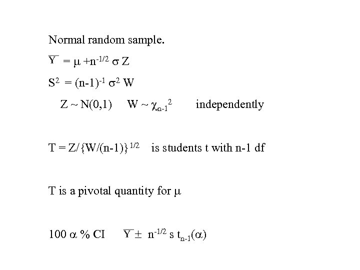Normal random sample. = +n-1/2 Z S 2 = (n-1)-1 2 W Z ~ N(0, 1) W ~ n-12 T = Z/{W/(n-1)}1/2 independently is students t with n-1 df T is a pivotal quantity for 100 % CI n-1/2 s tn-1( )

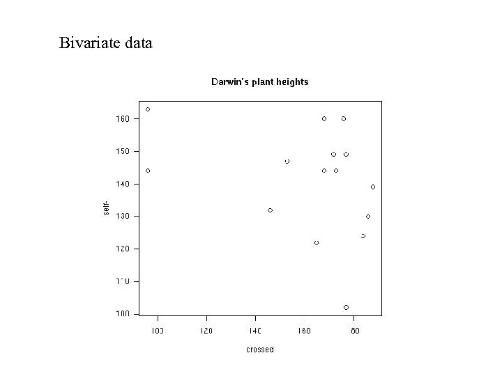Bivariate data

Bivariate distribution. cov(Y 1, Y 2) = E[(Y 1 - 1)(Y 2 - 2)] = 12 = cov(Y 2 , Y 1) Collect into a square array cov(Y, Y) = covariance matrix 2 by 2 variances, 11 and 22, on diagonal covariances, 12 and 21, off diagonal correlation = 12 / ( 11 22)

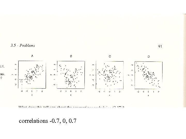correlations -0. 7, 0, 0. 7

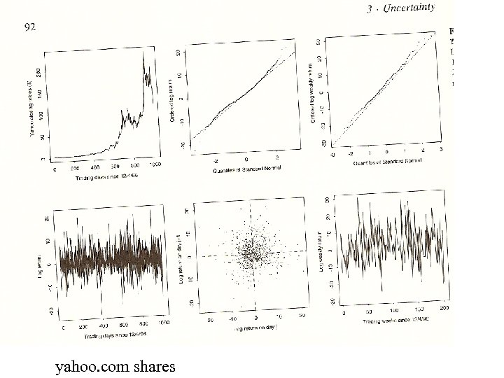yahoo. com shares

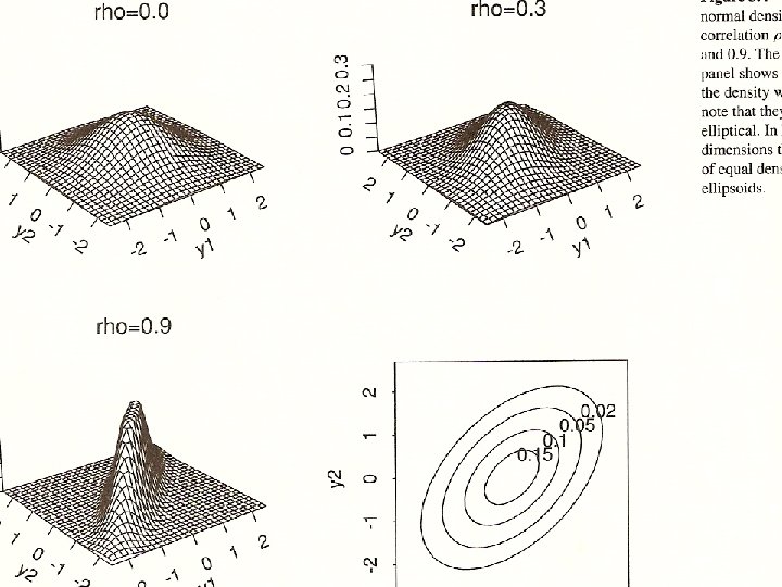
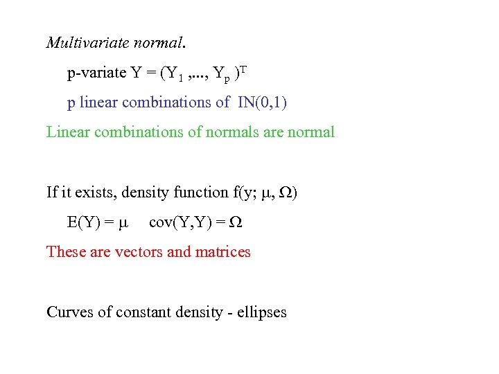Multivariate normal. p-variate Y = (Y 1 , . . . , Yp )T p linear combinations of IN(0, 1) Linear combinations of normals are normal If it exists, density function f(y; , ) E(Y) = cov(Y, Y) = These are vectors and matrices Curves of constant density - ellipses

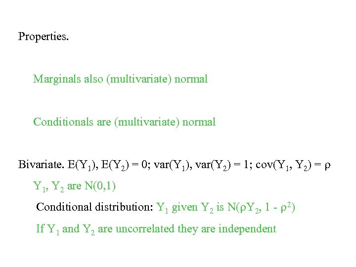Properties. Marginals also (multivariate) normal Conditionals are (multivariate) normal Bivariate. E(Y 1), E(Y 2) = 0; var(Y 1), var(Y 2) = 1; cov(Y 1, Y 2) = Y 1, Y 2 are N(0, 1) Conditional distribution: Y 1 given Y 2 is N( Y 2, 1 - 2) If Y 1 and Y 2 are uncorrelated they are independent

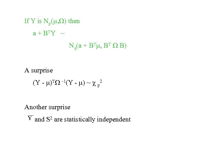If Y is Np( , ) then a + B TY ~ Nq(a + BT , BT B) A surprise (Y - )T -1(Y - ) ~ p 2 Another surprise and S 2 are statistically independent

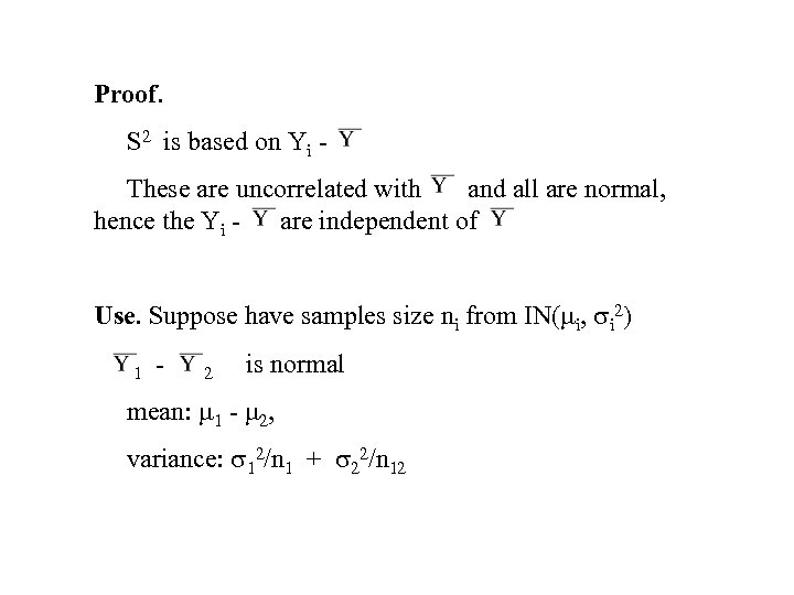Proof. S 2 is based on Yi These are uncorrelated with and all are normal, hence the Yi - are independent of Use. Suppose have samples size ni from IN( i, i 2) 1 - 2 is normal mean: 1 - 2, variance: 12/n 1 + 22/n 12

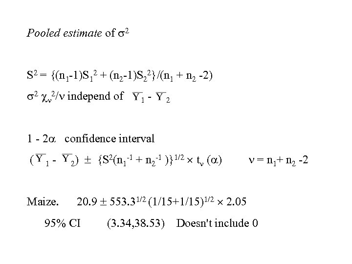Pooled estimate of 2 S 2 = {(n 1 -1)S 12 + (n 2 -1)S 22}/(n 1 + n 2 -2) 2 2/ independ of 1 - 2 confidence interval ( 1 - Maize. 2) {S 2(n 1 -1 + n 2 -1 )}1/2 t ( ) = n 1+ n 2 -2 20. 9 553. 31/2 (1/15+1/15)1/2 2. 05 95% CI (3. 34, 38. 53) Doesn't include 0

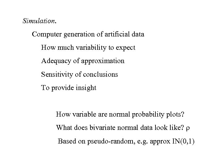Simulation. Computer generation of artificial data How much variability to expect Adequacy of approximation Sensitivity of conclusions To provide insight How variable are normal probability plots? What does bivariate normal data look like? Based on pseudo-random, e. g. approx IN(0, 1)

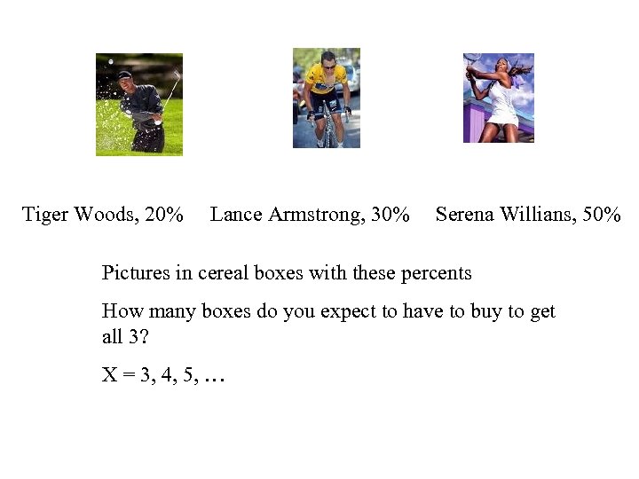Tiger Woods, 20% Lance Armstrong, 30% Serena Willians, 50% Pictures in cereal boxes with these percents How many boxes do you expect to have to buy to get all 3? X = 3, 4, 5, …

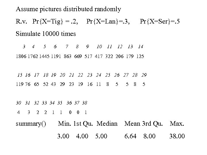Assume pictures distributed randomly R. v. Pr{X=Tig} =. 2, Pr{X=Lan}=. 3, Pr{X=Ser}=. 5 Simulate 10000 times 3 4 5 6 7 8 9 10 11 12 13 14 1806 1762 1445 1191 863 669 517 417 322 206 179 125 15 16 17 18 19 20 21 22 23 24 25 26 27 28 29 119 76 65 52 43 29 23 19 16 11 8 5 5 8 5 30 31 32 33 34 35 36 37 38 4 3 2 2 summary() 1 1 0 0 1 Min. 1 st Qu. Median Mean 3 rd Qu. Max. 3. 00 6. 64 38. 00 4. 00 5. 00 8. 00

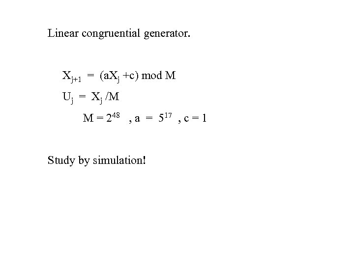Linear congruential generator. Xj+1 = (a. Xj +c) mod M Uj = Xj /M M = 248 , a = 517 , c = 1 Study by simulation!

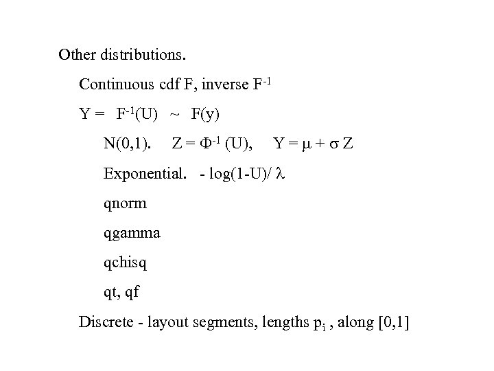Other distributions. Continuous cdf F, inverse F-1 Y = F-1(U) ~ F(y) N(0, 1). Z = -1 (U), Y= + Z Exponential. - log(1 -U)/ qnorm qgamma qchisq qt, qf Discrete - layout segments, lengths pi , along [0, 1]

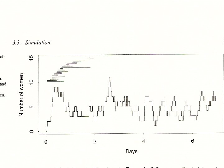
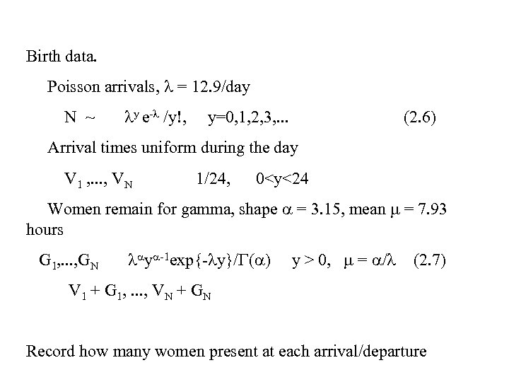Birth data. Poisson arrivals, = 12. 9/day N ~ y e- /y!, y=0, 1, 2, 3, . . . (2. 6) Arrival times uniform during the day V 1 , . . . , VN 1/24, 0 0, = / (2. 7) V 1 + G 1, . . . , VN + GN Record how many women present at each arrival/departure