Chapter 3 The Utility Function Approach to Consumer

Chapter 3 The Utility Function Approach to Consumer Choice Consumer’s Problem: Choose the BEST BUNDLE she/he can AFFORD. Breaking the problem into 2 stages: 1. Affordability problem – Budget Constraint: M = PSS + PFF 2. Best Bundle Problem – Utility Functions (older) or Indifference Curves (new) 3. We begin the analysis with the Affordability problem.

Rational Consumer Choice CHAPTER OUTLINE üThe opportunity set or budget constraint üConsumer preferences üThe best feasible bundle üAn application of the rational choice model BUDGET LIMITATIONS ØA bundle: a particular combination of two or more goods. ØBudget constraint: the set of all bundles that exactly exhaust the consumer’s income at given prices. ØIts slope is the negative of the price ratio of the two goods. 3 -2

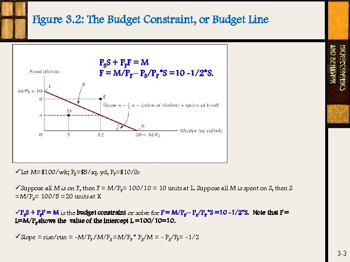Figure 3. 2: The Budget Constraint, or Budget Line PS S + P F F = M/PF – PS/PF *S =10 -1/2*S. üLet M=$100/wk; PS=$5/sq. yd, PF=$10/lb üSuppose all M is on F, then F = M/PF= 100/10 = 10 units at L. Suppose all M is spent on S, then S =M/PS= 100/5 =20 units at K üPSS + PFF = M is the budget constraint or solve for F = M/PF – PS/PF *S =10 -1/2*S. Note that F = L=M/PF shows the value of the intercept L =100/10=10. üSlope = rise/run = -M/PF /M/PS =M/PF * PS/M = - PS/PF= -1/2 3 -3

BUDGET SHIFTS DUE TO PRICE OR INCOME CHANGES 1. If the price of ONLY one good changes… – The slope of the budget constraint changes. 2. If the price of both goods change by the same proportion… – The budget constraint shifts parallel to the original one. 3. If income changes …. – The budget constraint shifts parallel to the original one. 3 -4

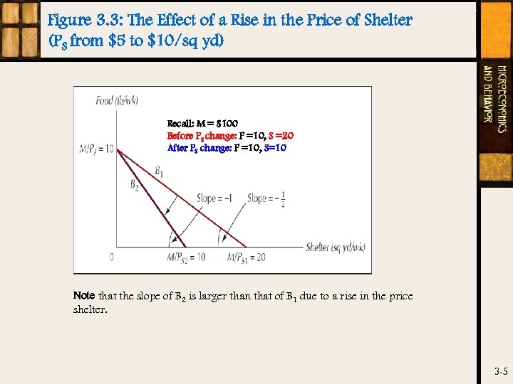Figure 3. 3: The Effect of a Rise in the Price of Shelter (PS from $5 to $10/sq yd) Recall: M = $100 Before PS change: F =10, S =20 After PS change: F =10, S=10 Note that the slope of B 2 is larger than that of B 1 due to a rise in the price shelter. 3 -5

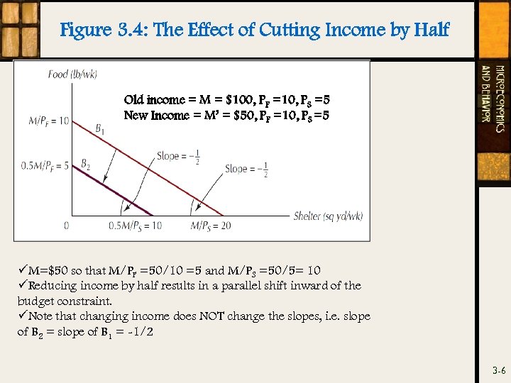Figure 3. 4: The Effect of Cutting Income by Half Old income = M = $100, PF =10, PS =5 New Income = M’ = $50, PF =10, PS =5 üM=$50 so that M/PF =50/10 =5 and M/PS =50/5= 10 üReducing income by half results in a parallel shift inward of the budget constraint. üNote that changing income does NOT change the slopes, i. e. slope of B 2 = slope of B 1 = -1/2 3 -6

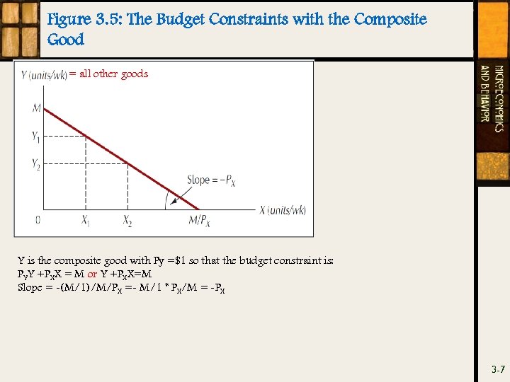Figure 3. 5: The Budget Constraints with the Composite Good = all other goods Y is the composite good with Py =$1 so that the budget constraint is: PYY +PXX = M or Y +PXX=M Slope = -(M/1)/M/PX =- M/1 * PX/M = -PX 3 -7

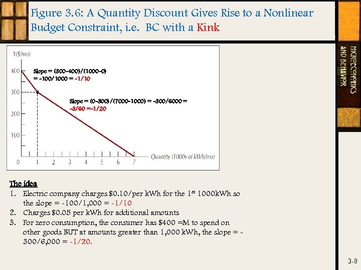Figure 3. 6: A Quantity Discount Gives Rise to a Nonlinear Budget Constraint, i. e. BC with a Kink Slope = (300 -400)/(1000 -0) = -100/1000 = -1/10 Slope = (0 -300)/(7000 -1000) = -300/6000 = -3/60 =-1/20 The idea 1. Electric company charges $0. 10/per k. Wh for the 1 st 1000 k. Wh so the slope = -100/1, 000 = -1/10 2. Charges $0. 05 per k. Wh for additional amounts 3. For zero consumption, the consumer has $400 =M to spend on other goods BUT at amounts greater than 1, 000 k. Wh, the slope = 300/6, 000 = -1/20. 3 -8

Properties of Preference Orderings ü Completeness: the consumer is able to rank all possible combinations of goods and services. ü More-Is-Better: other things equal, more of a good is preferred to less. ü Transitivity: for any three bundles A, B, and C, if he prefers A to B and prefers B to C, then he always prefers A to C. ü Convexity: mixtures of goods are preferable to extremes. 3 -9

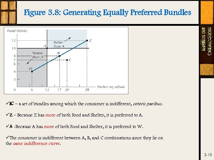Figure 3. 8: Generating Equally Preferred Bundles üIC – a set of bundles among which the consumer is indifferent, ceteris paribus. üZ – Because Z has more of both Food and Shelter, it is preferred to A. üA -Because A has more of both Food and Shelter, it is preferred to W. üThe consumer is indifferent between A, B, and C combinations since they lie on the same indifference curve. 3 -10

Indifference Curves ü Indifference curve: a set of bundles among which the consumer is indifferent. ü Indifference map: a representative sample of the set of a consumer’s indifference curves, used as a graphical summary of her preference ordering. Properties of Indifference Curves Indifference curves … 1. Are Ubiquitous. Any bundle has an indifference curve passing through it. 2. Are Downward-sloping. This comes from the “more-is-better” assumption. 3. Cannot cross. 4. Become less steep as we move downward and to the right along them. This property is implied by the convexity property of preferences. 3 -11

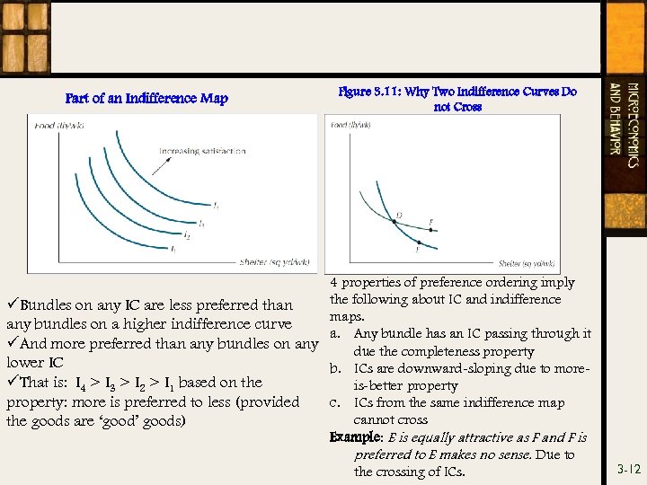Part of an Indifference Map Figure 3. 11: Why Two Indifference Curves Do not Cross 4 properties of preference ordering imply the following about IC and indifference üBundles on any IC are less preferred than maps. any bundles on a higher indifference curve a. Any bundle has an IC passing through it üAnd more preferred than any bundles on any due the completeness property lower IC b. ICs are downward-sloping due to moreüThat is: I 4 > I 3 > I 2 > I 1 based on the is-better property: more is preferred to less (provided c. ICs from the same indifference map cannot cross the goods are ‘good’ goods) Example: E is equally attractive as F and F is preferred to E makes no sense. Due to the crossing of ICs. 3 -12

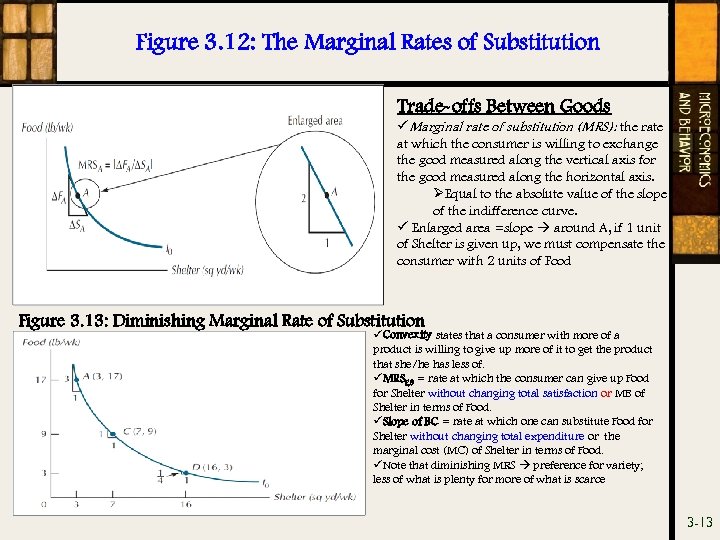Figure 3. 12: The Marginal Rates of Substitution Trade-offs Between Goods üMarginal rate of substitution (MRS): the rate at which the consumer is willing to exchange the good measured along the vertical axis for the good measured along the horizontal axis. ØEqual to the absolute value of the slope of the indifference curve. ü Enlarged area =slope around A, if 1 unit of Shelter is given up, we must compensate the consumer with 2 units of Food Figure 3. 13: Diminishing Marginal Rate of Substitution üConvexity states that a consumer with more of a product is willing to give up more of it to get the product that she/he has less of. üMRSF, S = rate at which the consumer can give up Food for Shelter without changing total satisfaction or MB of Shelter in terms of Food. üSlope of BC = rate at which one can substitute Food for Shelter without changing total expenditure or the marginal cost (MC) of Shelter in terms of Food. üNote that diminishing MRS preference for variety; less of what is plenty for more of what is scarce 3 -13

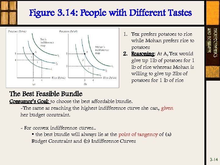Figure 3. 14: People with Different Tastes 1. Tex prefers potatoes to rice while Mohan prefers rice to potatoes 2. Reasoning: At A, Tex would give up 1 lb of potatoes for 1 lb of rice whereas Mohan is willing to give up 2 lbs of potatoes for 1 lb of rice The Best Feasible Bundle Consumer’s Goal: to choose the best affordable bundle. -The same as reaching the highest indifference curve she can, given her budget constraint. - For convex indifference curves. . § the best bundle will always lie at the point of tangency of (a) Budget Constraint and (b) Indifference Curves 3 -14

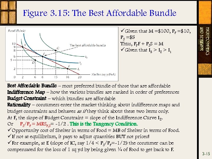Figure 3. 15: The Best Affordable Bundle üGiven that M =$100, PF =$10, PS =$5 Thus, PFF + PSS = M üGiven that I 3 > I 2 > I 1 Best Affordable Bundle – most preferred bundle of those that are affordable Indifference Map – how the various bundles are ranked in order of preferences Budget Constraint – which bundles are affordable Rationality – consumers enter the market thinking about indifference maps and budget constraints and behaves as if they think about these two items only. At F, the slope of Budget Constraint = slope of the Indifference Curve I 2. Or PS/PF = MRSF, S= -1/2. This is the Tangency Condition. üOpportunity cost of Shelter in terms of Food = MB of Shelter in terms of Food. üIf not at equilibrium, it pays to adjust quantities BUT not prices! üFor example, at E (slope of IC, say 1/4 < PS/PF=-1/2) the consumer can be compensated for the loss of 1 sq yd by being given ¼ of Food to get back to F. 3 -15

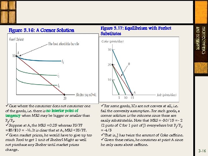Figure 3. 16: A Corner Solution üCase where the consumer does not consumer one of the goods, i. e. there is no interior point of tangency when MRS may be bigger or smaller than PS/PF. üSuppose at A, the MRS =0. 25 whereas PS/PF =$5/$10 = -½. It is clear that at A, MRS

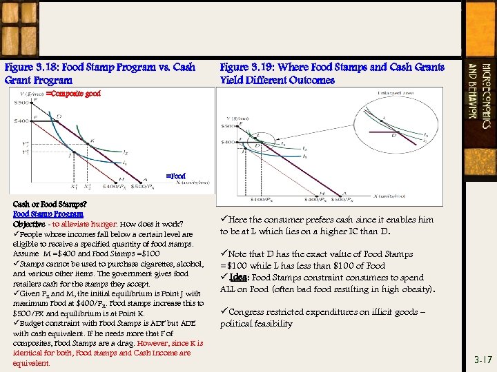Figure 3. 18: Food Stamp Program vs. Cash Grant Program Figure 3. 19: Where Food Stamps and Cash Grants Yield Different Outcomes =Composite good =Food Cash or Food Stamps? Food Stamp Program Objective - to alleviate hunger. How does it work? üPeople whose incomes fall below a certain level are eligible to receive a specified quantity of food stamps. Assume M =$400 and Food Stamps =$100 üStamps cannot be used to purchase cigarettes, alcohol, and various other items. The government gives food retailers cash for the stamps they accept. üGiven PX and M, the initial equilibrium is Point J with maximum Food at $400/PX. Food stamps increase this to $500/PX and equilibrium is at Point K. üBudget constraint with Food Stamps is ADF but ADE with cash equivalent. If he needs more that F of composites, Food Stamps are a drag. However, since K is identical for both, Food stamps and Cash Income are equivalent. üHere the consumer prefers cash since it enables him to be at L which lies on a higher IC than D. üNote that D has the exact value of Food Stamps =$100 while L has less than $100 of Food ü. Idea: Food Stamps constraint consumers to spend ALL on Food (often bad food resulting in high obesity). üCongress restricted expenditures on illicit goods – political feasibility 3 -17

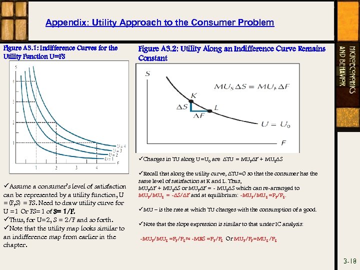Appendix: Utility Approach to the Consumer Problem Figure A 3. 1: Indifference Curves for the Utility Function U=FS Figure A 3. 2: Utility Along an Indifference Curve Remains Constant üChanges in TU along U=U 0 are ∆TU = MUF∆F + MUS∆S üAssume a consumer’s level of satisfaction can be represented by a utility function, U =(F, S) = FS. Need to draw utility curve for U =1 Or FS=1 of S= 1/F. üThus, for U=2, S = 2/F and so forth. üNote that the utility map looks similar to an indifference map from earlier in the chapter. üRecall that along the utility curve, ∆TU=0 so that the consumer has the same level of satisfaction at K and L. Thus, MUF∆F + MUS∆S or MUF∆F = - MUS∆S which can re-arranged to MUF/MUS = -∆S/∆F and at equilibrium: -MUF/MUS =PF/PS. üMU – is the rate at which TU changes with the consumption of a good. üNote that the slope expression is similar to that under IC analysis: -MUF/MUS =PF/PS ≈ -MRS =PF/PS Or MUF/PF=MUS /PS 3 -18

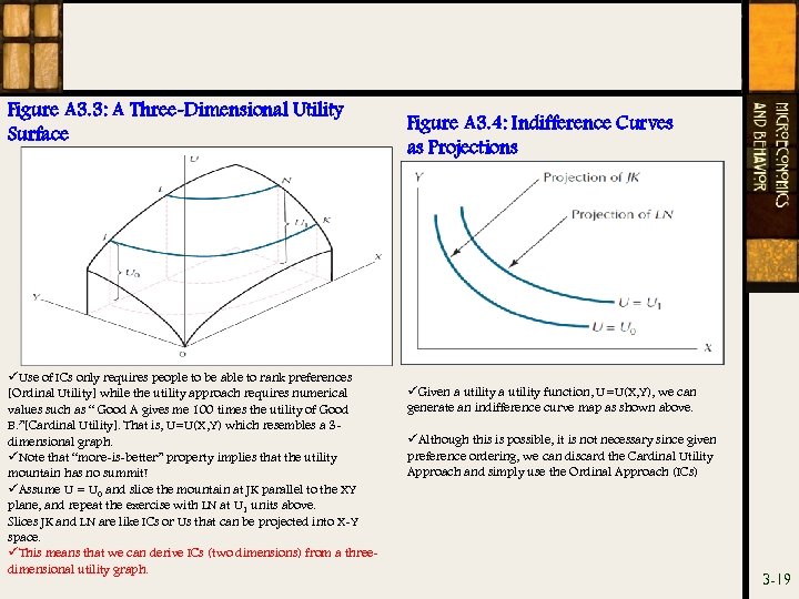Figure A 3. 3: A Three-Dimensional Utility Surface üUse of ICs only requires people to be able to rank preferences [Ordinal Utility] while the utility approach requires numerical values such as “ Good A gives me 100 times the utility of Good B. ”[Cardinal Utility]. That is, U=U(X, Y) which resembles a 3 dimensional graph. üNote that “more-is-better” property implies that the utility mountain has no summit! üAssume U = U 0 and slice the mountain at JK parallel to the XY plane, and repeat the exercise with LN at U 1 units above. Slices JK and LN are like ICs or Us that can be projected into X-Y space. üThis means that we can derive ICs (two dimensions) from a threedimensional utility graph. Figure A 3. 4: Indifference Curves as Projections üGiven a utility function, U=U(X, Y), we can generate an indifference curve map as shown above. üAlthough this is possible, it is not necessary since given preference ordering, we can discard the Cardinal Utility Approach and simply use the Ordinal Approach (ICs) 3 -19

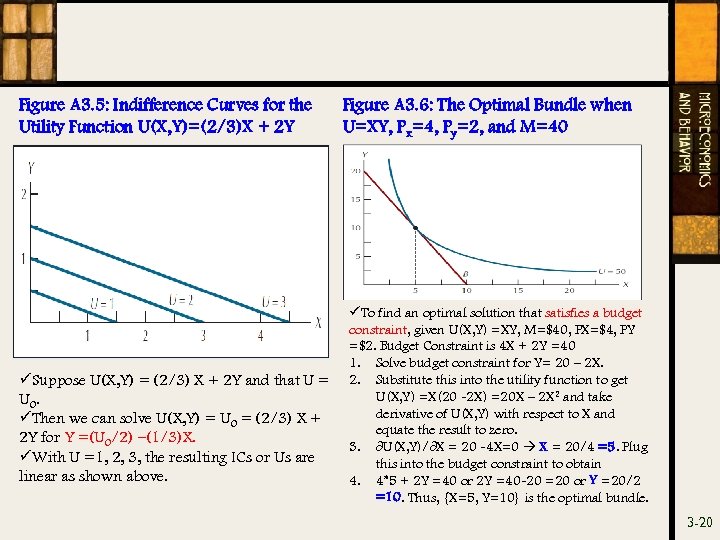Figure A 3. 5: Indifference Curves for the Utility Function U(X, Y)=(2/3)X + 2 Y üSuppose U(X, Y) = (2/3) X + 2 Y and that U = U 0. üThen we can solve U(X, Y) = U 0 = (2/3) X + 2 Y for Y =(U 0/2) –(1/3)X. üWith U =1, 2, 3, the resulting ICs or Us are linear as shown above. Figure A 3. 6: The Optimal Bundle when U=XY, Px=4, Py=2, and M=40 üTo find an optimal solution that satisfies a budget constraint, given U(X, Y) =XY, M=$40, PX=$4, PY =$2. Budget Constraint is 4 X + 2 Y =40 1. Solve budget constraint for Y= 20 – 2 X. 2. Substitute this into the utility function to get U(X, Y) =X(20 -2 X) =20 X – 2 X 2 and take derivative of U(X, Y) with respect to X and equate the result to zero. 3. ∂U(X, Y)/∂X = 20 -4 X=0 X = 20/4 =5. Plug this into the budget constraint to obtain 4. 4*5 + 2 Y =40 or 2 Y =40 -20 =20 or Y =20/2 =10. Thus, {X=5, Y=10} is the optimal bundle. 3 -20

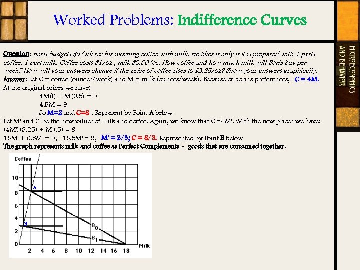Worked Problems: Indifference Curves Question: Boris budgets $9/wk for his morning coffee with milk. He likes it only if it is prepared with 4 parts coffee, 1 part milk. Coffee costs $1/oz , milk $0. 50/oz. How coffee and how much milk will Boris buy per week? How will your answers change if the price of coffee rises to $3. 25/oz? Show your answers graphically. Answer: Let C = coffee (ounces/week) and M = milk (ounces/week). Because of Boris's preferences, C = 4 M. At the original prices we have: 4 M(l) + M(0. 5) = 9 4. 5 M = 9 So M=2 and C=8. Represent by Point A below Let M' and C' be the new values of milk and coffee. Again, we know that C'=4 M'. With the new prices we have: (4 M')(3. 25) + M'(. 5) = 9 13 M' + 0. 5 M' = 9, 13. 5 M' = 9, M' = 2/3; C = 8/3. Represented by Point B below The graph represents milk and coffee as Perfect Complements - goods that are consumed together. A B

Worked Problem: Utility Function Approach Question: Tom spends all his $100 weekly income on two goods, X and Y. His utility function is given by U(X, Y)=XY. If PX =4 and PY =10, how much of each good should he buy? Budget Constraint: PXX + PYY = M 4 X + 10 Y =$100 Answer: üSolve the budget constraint, 100 = 4 X + l 0 Y, to get Y = 10 0. 4 X, then substitute into the utility function to get U = XY = X(10 0. 4 X ) = 10 X 0. 4 X 2. üEquating ∂U/∂X to zero we have 10 0. 8 X = 0, which solves for X = 12. 5. üSubstituting back into the budget constraint and solving for Y, we get Y = 5.