Chapter 3 Interval Estimation and Hypothesis Testing Walter

Chapter 3 Interval Estimation and Hypothesis Testing Walter R. Paczkowski Rutgers University Principles of Econometrics, 4 th Edition Chapter 3: Interval Estimation and Hypothesis Testing Page 1

Chapter Contents 3. 1 Interval Estimation 3. 2 Hypothesis Tests 3. 3 Rejection Regions for Specific Alternatives 3. 4 Examples of Hypothesis Tests 3. 5 The p-value 3. 6 Linear Combinations of Parameters Principles of Econometrics, 4 th Edition Chapter 3: Interval Estimation and Hypothesis Testing Page 2

3. 1 Interval Estimation Principles of Econometrics, 4 th Edition Chapter 3: Interval Estimation and Hypothesis Testing Page 3

3. 1 Interval Estimation There are two types of estimates – Point estimates • The estimate b 2 is a point estimate of the unknown population parameter in the regression model. – Interval estimates • Interval estimation proposes a range of values in which the true parameter is likely to fall • Providing a range of values gives a sense of what the parameter value might be, and the precision with which we have estimated it • Such intervals are often called confidence intervals. – We prefer to call them interval estimates because the term ‘‘confidence’’ is widely misunderstood and misused Principles of Econometrics, 4 th Edition Chapter 3: Interval Estimation and Hypothesis Testing Page 4

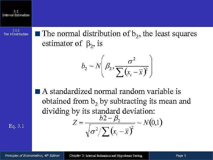3. 1 Interval Estimation 3. 1. 1 The t-Distribution The normal distribution of b 2, the least squares estimator of β 2, is A standardized normal random variable is obtained from b 2 by subtracting its mean and dividing by its standard deviation: Eq. 3. 1 Principles of Econometrics, 4 th Edition Chapter 3: Interval Estimation and Hypothesis Testing Page 5

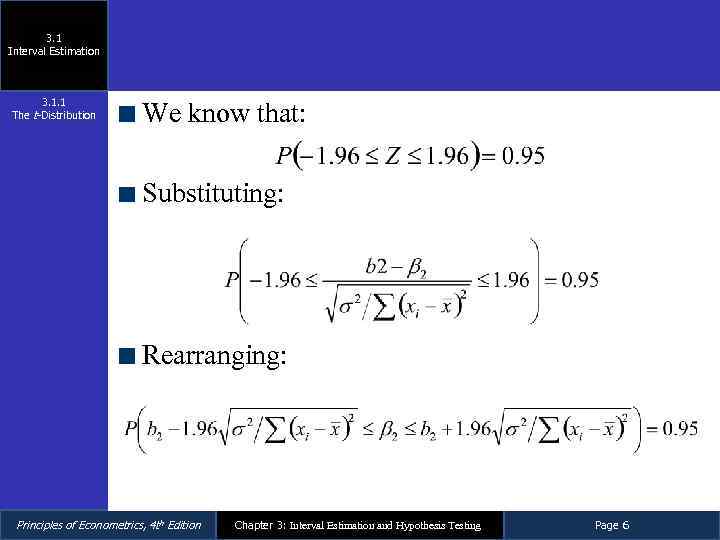3. 1 Interval Estimation 3. 1. 1 The t-Distribution We know that: Substituting: Rearranging: Principles of Econometrics, 4 th Edition Chapter 3: Interval Estimation and Hypothesis Testing Page 6

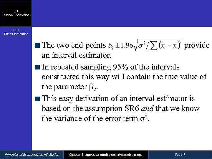3. 1 Interval Estimation 3. 1. 1 The t-Distribution The two end-points provide an interval estimator. In repeated sampling 95% of the intervals constructed this way will contain the true value of the parameter β 2. This easy derivation of an interval estimator is based on the assumption SR 6 and that we know the variance of the error term σ2. Principles of Econometrics, 4 th Edition Chapter 3: Interval Estimation and Hypothesis Testing Page 7

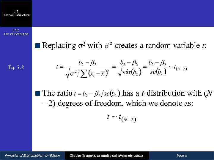3. 1 Interval Estimation 3. 1. 1 The t-Distribution Replacing σ2 with creates a random variable t: Eq. 3. 2 The ratio has a t-distribution with (N – 2) degrees of freedom, which we denote as: Principles of Econometrics, 4 th Edition Chapter 3: Interval Estimation and Hypothesis Testing Page 8

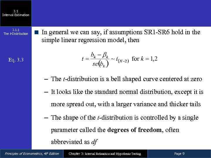3. 1 Interval Estimation 3. 1. 1 The t-Distribution In general we can say, if assumptions SR 1 -SR 6 hold in the simple linear regression model, then Eq. 3. 3 – The t-distribution is a bell shaped curve centered at zero – It looks like the standard normal distribution, except it is more spread out, with a larger variance and thicker tails – The shape of the t-distribution is controlled by a single parameter called the degrees of freedom, often abbreviated as df Principles of Econometrics, 4 th Edition Chapter 3: Interval Estimation and Hypothesis Testing Page 9

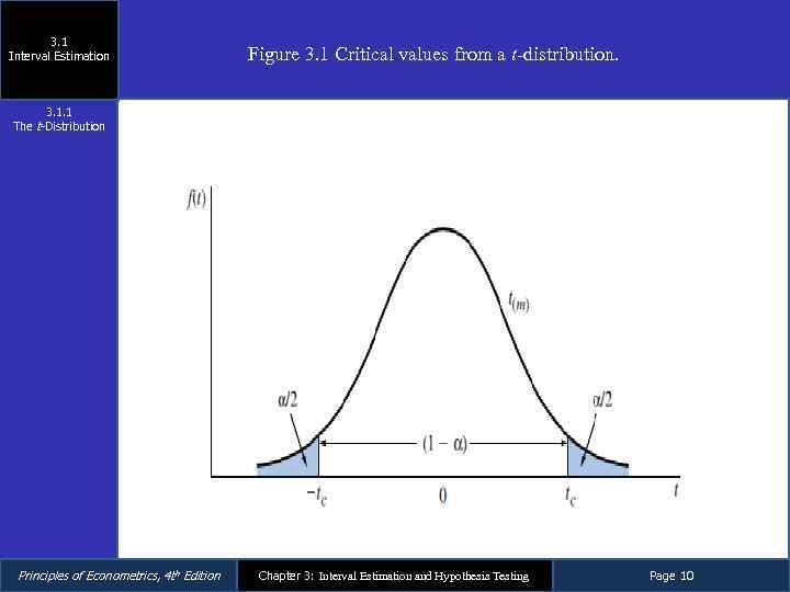3. 1 Interval Estimation Figure 3. 1 Critical values from a t-distribution. 3. 1. 1 The t-Distribution Principles of Econometrics, 4 th Edition Chapter 3: Interval Estimation and Hypothesis Testing Page 10

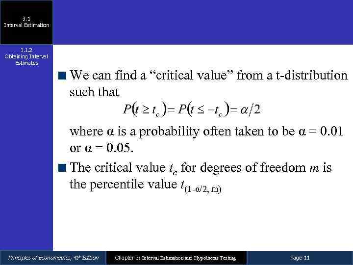3. 1 Interval Estimation 3. 1. 2 Obtaining Interval Estimates We can find a “critical value” from a t-distribution such that where α is a probability often taken to be α = 0. 01 or α = 0. 05. The critical value tc for degrees of freedom m is the percentile value t(1 -α/2, m) Principles of Econometrics, 4 th Edition Chapter 3: Interval Estimation and Hypothesis Testing Page 11

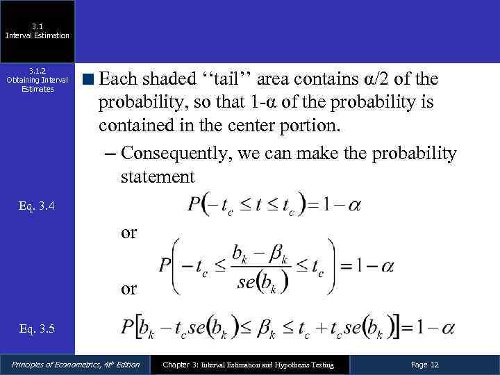3. 1 Interval Estimation 3. 1. 2 Obtaining Interval Estimates Each shaded ‘‘tail’’ area contains α/2 of the probability, so that 1 -α of the probability is contained in the center portion. – Consequently, we can make the probability statement Eq. 3. 4 or or Eq. 3. 5 Principles of Econometrics, 4 th Edition Chapter 3: Interval Estimation and Hypothesis Testing Page 12

3. 1 Interval Estimation 3. 1. 2 Obtaining Interval Estimates When bk and se(bk) are estimated values (numbers), based on a given sample of data, then bk ± tcse(bk) is called a 100(1 -α)% interval estimate of bk. – Equivalently it is called a 100(1 -α)% confidence interval. – Usually α = 0. 01 or α = 0. 05, so that we obtain a 99% confidence interval or a 95% confidence interval. Principles of Econometrics, 4 th Edition Chapter 3: Interval Estimation and Hypothesis Testing Page 13

3. 1 Interval Estimation 3. 1. 2 Obtaining Interval Estimates The interpretation of confidence intervals requires a great deal of care – The properties of the interval estimation procedure are based on the notion of repeated sampling – Any one interval estimate, based on one sample of data, may or may not contain the true parameter βk, and because βk is unknown, we will never know whether it does or does not – When ‘‘confidence intervals’’ are discussed, remember that our confidence is in the procedure used to construct the interval estimate; it is not in any one interval estimate calculated from a sample of data Principles of Econometrics, 4 th Edition Chapter 3: Interval Estimation and Hypothesis Testing Page 14

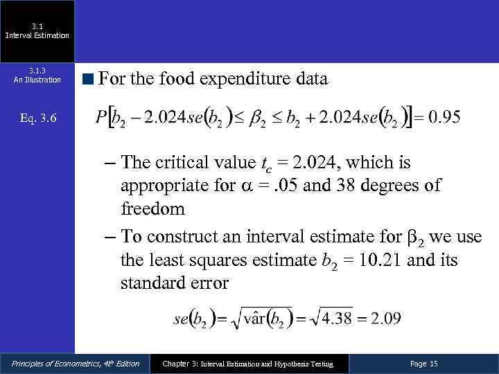3. 1 Interval Estimation 3. 1. 3 An Illustration For the food expenditure data Eq. 3. 6 – The critical value tc = 2. 024, which is appropriate for =. 05 and 38 degrees of freedom – To construct an interval estimate for 2 we use the least squares estimate b 2 = 10. 21 and its standard error Principles of Econometrics, 4 th Edition Chapter 3: Interval Estimation and Hypothesis Testing Page 15

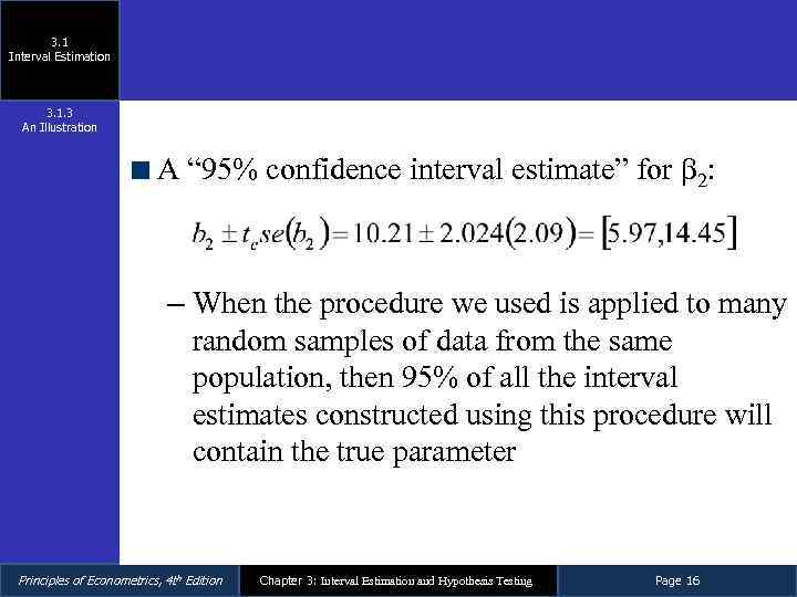3. 1 Interval Estimation 3. 1. 3 An Illustration A “ 95% confidence interval estimate” for 2: – When the procedure we used is applied to many random samples of data from the same population, then 95% of all the interval estimates constructed using this procedure will contain the true parameter Principles of Econometrics, 4 th Edition Chapter 3: Interval Estimation and Hypothesis Testing Page 16

3. 1 Interval Estimation 3. 1. 3 An Illustration Is β 2 actually in the interval [5. 97, 14. 45]? – We do not know, and we will never know – What we do know is that when the procedure we used is applied to many random samples of data from the same population, then 95% of all the interval estimates constructed using this procedure will contain the true parameter – The interval estimation procedure ‘‘works’’ 95% of the time • What we can say about the interval estimate based on our one sample is that, given the reliability of the procedure, we would be ‘‘surprised’’ if β 2 is not in the interval [5. 97, 14. 45]. Principles of Econometrics, 4 th Edition Chapter 3: Interval Estimation and Hypothesis Testing Page 17

3. 1 Interval Estimation 3. 1. 3 An Illustration What is the usefulness of an interval estimate of β 2? – When reporting regression results we always give a point estimate, such as b 2 = 10. 21 – However, the point estimate alone gives no sense of its reliability – Thus, we might also report an interval estimate • Interval estimates incorporate both the point estimate and the standard error of the estimate, which is a measure of the variability of the least squares estimator Principles of Econometrics, 4 th Edition Chapter 3: Interval Estimation and Hypothesis Testing Page 18

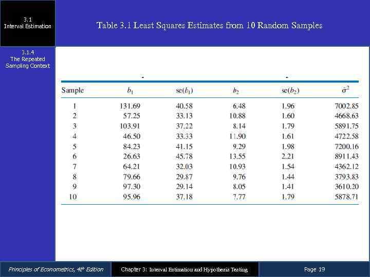3. 1 Interval Estimation Table 3. 1 Least Squares Estimates from 10 Random Samples 3. 1. 4 The Repeated Sampling Context Principles of Econometrics, 4 th Edition Chapter 3: Interval Estimation and Hypothesis Testing Page 19

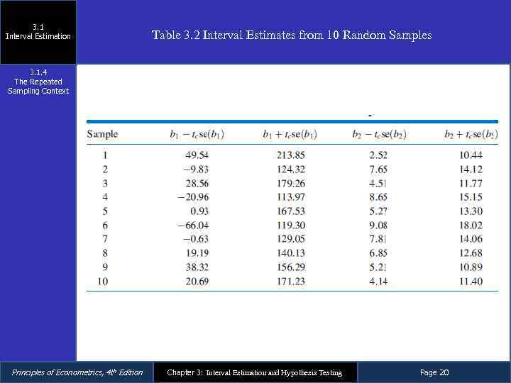3. 1 Interval Estimation Table 3. 2 Interval Estimates from 10 Random Samples 3. 1. 4 The Repeated Sampling Context Principles of Econometrics, 4 th Edition Chapter 3: Interval Estimation and Hypothesis Testing Page 20

3. 2 Hypothesis Tests Principles of Econometrics, 4 th Edition Chapter 3: Interval Estimation and Hypothesis Testing Page 21

3. 2 Hypothesis Tests Hypothesis testing procedures compare a conjecture we have about a population to the information contained in a sample of data – Given an economic and statistical model, hypotheses are formed about economic behavior. – These hypotheses are then represented as statements about model parameters – Hypothesis tests use the information about a parameter that is contained in a sample of data, its least squares point estimate, and its standard error, to draw a conclusion about the hypothesis Principles of Econometrics, 4 th Edition Chapter 3: Interval Estimation and Hypothesis Testing Page 22

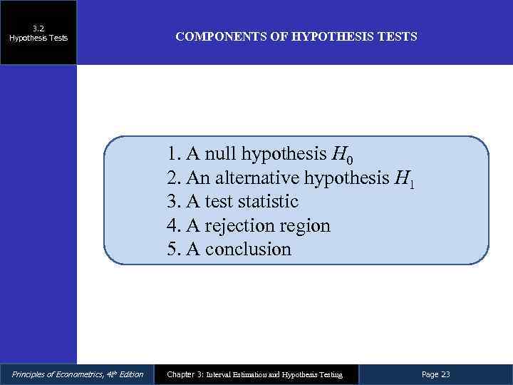3. 2 Hypothesis Tests COMPONENTS OF HYPOTHESIS TESTS 1. A null hypothesis H 0 2. An alternative hypothesis H 1 3. A test statistic 4. A rejection region 5. A conclusion Principles of Econometrics, 4 th Edition Chapter 3: Interval Estimation and Hypothesis Testing Page 23

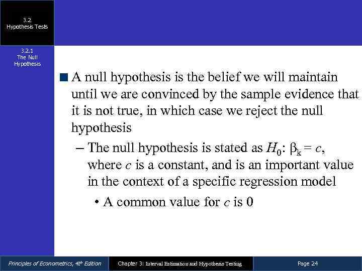3. 2 Hypothesis Tests 3. 2. 1 The Null Hypothesis A null hypothesis is the belief we will maintain until we are convinced by the sample evidence that it is not true, in which case we reject the null hypothesis – The null hypothesis is stated as H 0 : βk = c, where c is a constant, and is an important value in the context of a specific regression model • A common value for c is 0 Principles of Econometrics, 4 th Edition Chapter 3: Interval Estimation and Hypothesis Testing Page 24

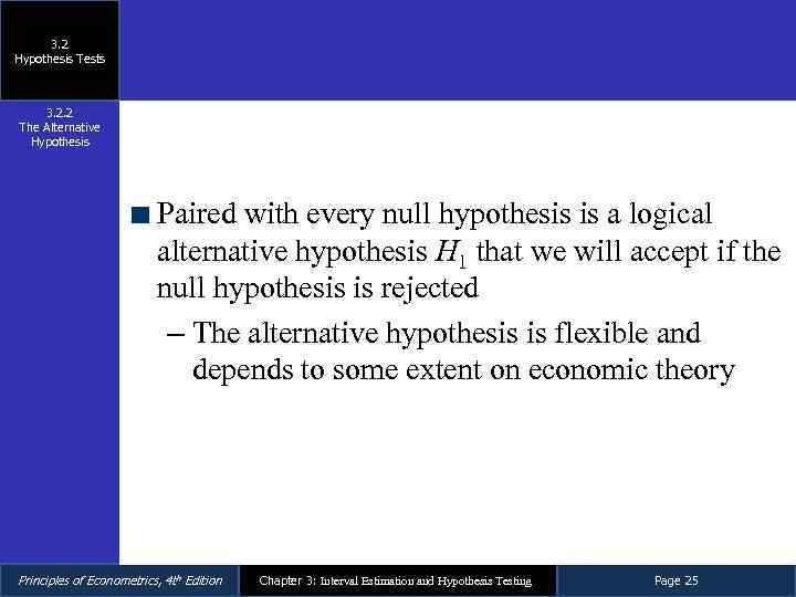3. 2 Hypothesis Tests 3. 2. 2 The Alternative Hypothesis Paired with every null hypothesis is a logical alternative hypothesis H 1 that we will accept if the null hypothesis is rejected – The alternative hypothesis is flexible and depends to some extent on economic theory Principles of Econometrics, 4 th Edition Chapter 3: Interval Estimation and Hypothesis Testing Page 25

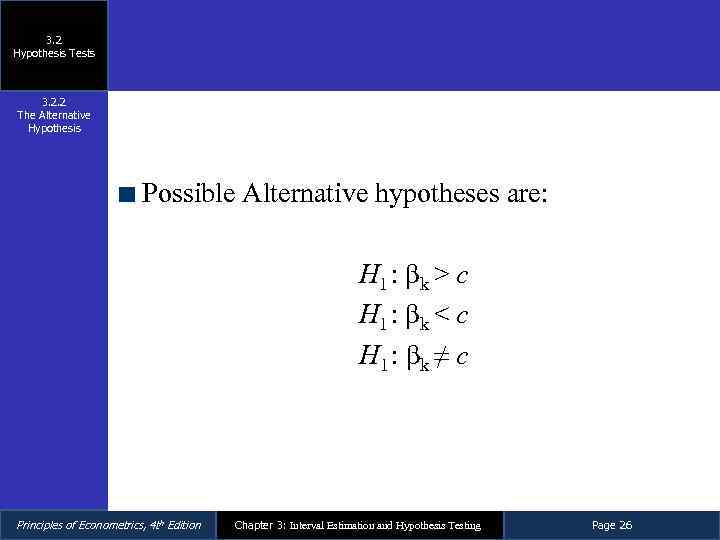3. 2 Hypothesis Tests 3. 2. 2 The Alternative Hypothesis Possible Alternative hypotheses are: H 1 : β k > c H 1 : β k < c H 1 : β k ≠ c Principles of Econometrics, 4 th Edition Chapter 3: Interval Estimation and Hypothesis Testing Page 26

3. 2 Hypothesis Tests 3. 2. 3 The Test Statistic Based on the value of a test statistic we decide either to reject the null hypothesis or not to reject it – A test statistic has a special characteristic: its probability distribution is completely known when the null hypothesis is true, and it has some other distribution if the null hypothesis is not true Principles of Econometrics, 4 th Edition Chapter 3: Interval Estimation and Hypothesis Testing Page 27

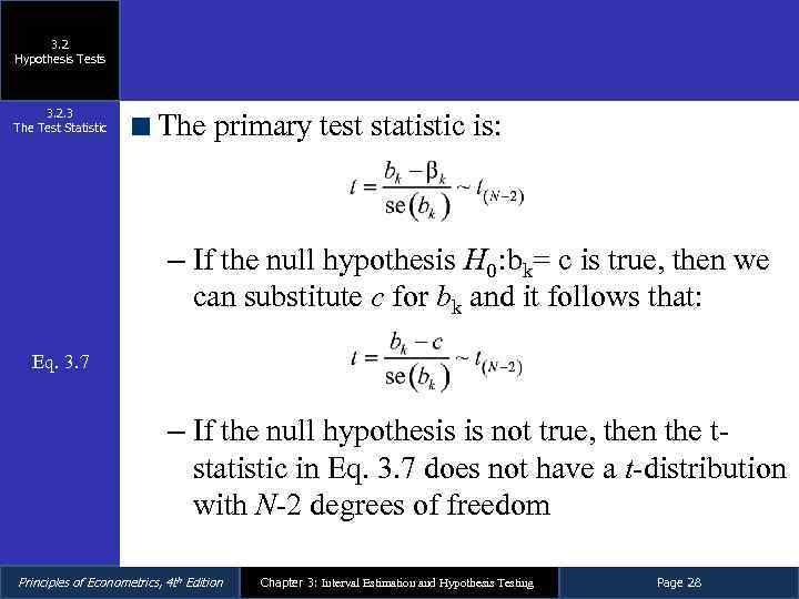3. 2 Hypothesis Tests 3. 2. 3 The Test Statistic The primary test statistic is: – If the null hypothesis H 0 : bk= c is true, then we can substitute c for bk and it follows that: Eq. 3. 7 – If the null hypothesis is not true, then the tstatistic in Eq. 3. 7 does not have a t-distribution with N-2 degrees of freedom Principles of Econometrics, 4 th Edition Chapter 3: Interval Estimation and Hypothesis Testing Page 28

3. 2 Hypothesis Tests 3. 2. 4 The Rejection Region The rejection region depends on the form of the alternative – It is the range of values of the test statistic that leads to rejection of the null hypothesis – It is possible to construct a rejection region only if we have: • A test statistic whose distribution is known when the null hypothesis is true • An alternative hypothesis • A level of significance Principles of Econometrics, 4 th Edition Chapter 3: Interval Estimation and Hypothesis Testing Page 29

3. 2 Hypothesis Tests 3. 2. 4 The Rejection Region The rejection region consists of values that are unlikely and that have low probability of occurring when the null hypothesis is true – The chain of logic is: ‘‘If a value of the test statistic is obtained that falls in a region of low probability, then it is unlikely that the test statistic has the assumed distribution, and thus it is unlikely that the null hypothesis is true’’ Principles of Econometrics, 4 th Edition Chapter 3: Interval Estimation and Hypothesis Testing Page 30

3. 2 Hypothesis Tests 3. 2. 4 The Rejection Region If the alternative hypothesis is true, then values of the test statistic will tend to be unusually large or unusually small – The terms ‘‘large’’ and ‘‘small’’ are determined by choosing a probability α, called the level of significance of the test, which provides a meaning for ‘‘an unlikely event’’ – The level of significance of the test α is usually chosen to be 0. 01, 0. 05 or 0. 10 Principles of Econometrics, 4 th Edition Chapter 3: Interval Estimation and Hypothesis Testing Page 31

3. 2 Hypothesis Tests 3. 2. 4 The Rejection Region We could commit two types of error – If we reject the null hypothesis when it is true, then we commit what is called a Type error • The level of significance of a test is the probability of committing a Type I error • P(Type I error) = α – If we do not reject a null hypothesis that is false, then we have committed a Type II error Principles of Econometrics, 4 th Edition Chapter 3: Interval Estimation and Hypothesis Testing Page 32

3. 2 Hypothesis Tests 3. 2. 5 Conclusion Do you reject the null hypothesis, or do you not reject the null hypothesis? – Avoid saying that you ‘‘accept’’ the null hypothesis – Make it standard practice to say what the conclusion means in the economic context of the problem you are working on and the economic significance of the finding Principles of Econometrics, 4 th Edition Chapter 3: Interval Estimation and Hypothesis Testing Page 33

3. 3 Rejection Regions for Specific Alternatives Principles of Econometrics, 4 th Edition Chapter 3: Interval Estimation and Hypothesis Testing Page 34

3. 3 Rejection Regions for Specific Alternatives To have a rejection region for a null hypothesis, we need: 1. A test statistic 2. A specific alternative 3. A level of significance, α, for the test Principles of Econometrics, 4 th Edition Chapter 3: Interval Estimation and Hypothesis Testing Page 35

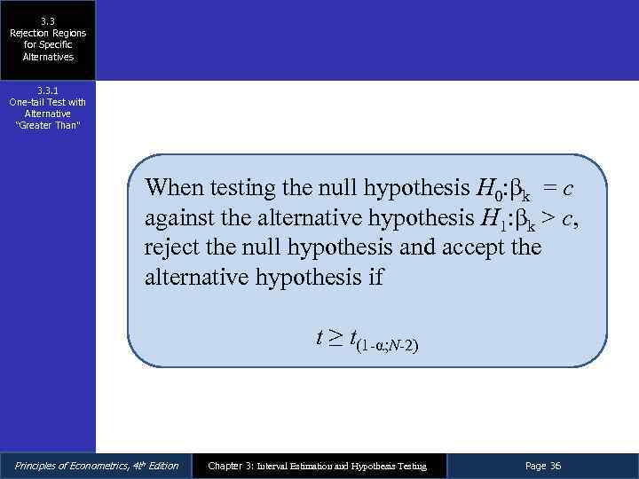3. 3 Rejection Regions for Specific Alternatives 3. 3. 1 One-tail Test with Alternative “Greater Than” When testing the null hypothesis H 0: βk = c against the alternative hypothesis H 1: βk > c, reject the null hypothesis and accept the alternative hypothesis if t ≥ t(1 -α; N-2) Principles of Econometrics, 4 th Edition Chapter 3: Interval Estimation and Hypothesis Testing Page 36

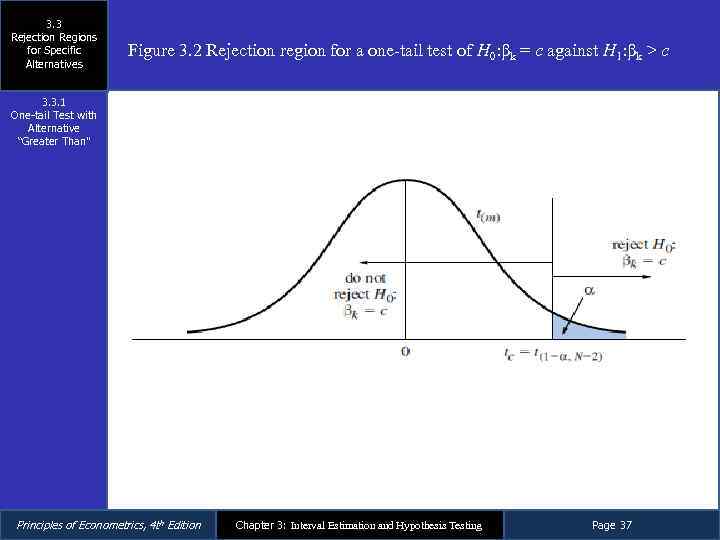3. 3 Rejection Regions for Specific Alternatives Figure 3. 2 Rejection region for a one-tail test of H 0: βk = c against H 1: βk > c 3. 3. 1 One-tail Test with Alternative “Greater Than” Principles of Econometrics, 4 th Edition Chapter 3: Interval Estimation and Hypothesis Testing Page 37

3. 3 Rejection Regions for Specific Alternatives 3. 3. 2 One-tail Test with Alternative “Less Than” When testing the null hypothesis H 0: βk = c against the alternative hypothesis H 1: βk < c, reject the null hypothesis and accept the alternative hypothesis if t ≤ t(1 -α; N-2) Principles of Econometrics, 4 th Edition Chapter 3: Interval Estimation and Hypothesis Testing Page 38

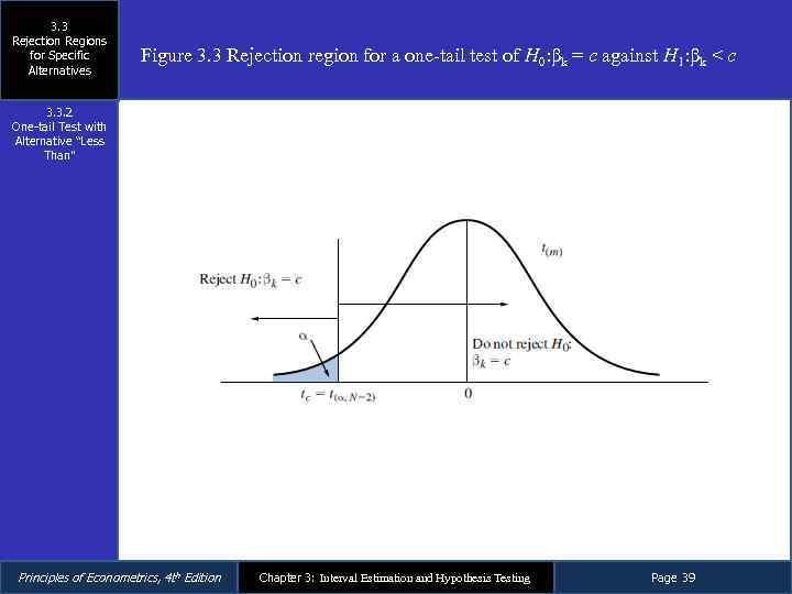3. 3 Rejection Regions for Specific Alternatives Figure 3. 3 Rejection region for a one-tail test of H 0: βk = c against H 1: βk < c 3. 3. 2 One-tail Test with Alternative “Less Than” Principles of Econometrics, 4 th Edition Chapter 3: Interval Estimation and Hypothesis Testing Page 39

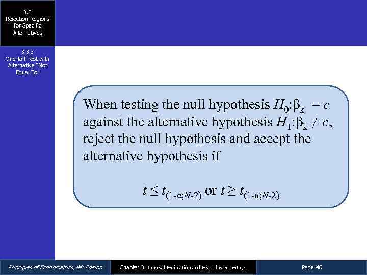3. 3 Rejection Regions for Specific Alternatives 3. 3. 3 One-tail Test with Alternative “Not Equal To” When testing the null hypothesis H 0: βk = c against the alternative hypothesis H 1: βk ≠ c, reject the null hypothesis and accept the alternative hypothesis if t ≤ t(1 -α; N-2) or t ≥ t(1 -α; N-2) Principles of Econometrics, 4 th Edition Chapter 3: Interval Estimation and Hypothesis Testing Page 40

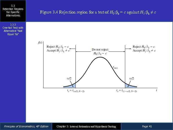3. 3 Rejection Regions for Specific Alternatives Figure 3. 4 Rejection region for a test of H 0: βk = c against H 1: βk ≠ c 3. 3. 3 One-tail Test with Alternative “Not Equal To” Principles of Econometrics, 4 th Edition Chapter 3: Interval Estimation and Hypothesis Testing Page 41

3. 4 Examples of Hypothesis Tests Principles of Econometrics, 4 th Edition Chapter 3: Interval Estimation and Hypothesis Testing Page 42

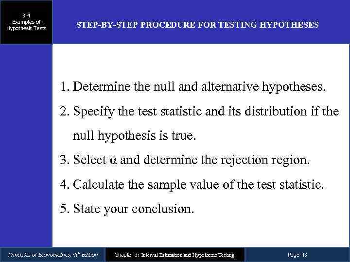3. 4 Examples of Hypothesis Tests STEP-BY-STEP PROCEDURE FOR TESTING HYPOTHESES 1. Determine the null and alternative hypotheses. 2. Specify the test statistic and its distribution if the null hypothesis is true. 3. Select α and determine the rejection region. 4. Calculate the sample value of the test statistic. 5. State your conclusion. Principles of Econometrics, 4 th Edition Chapter 3: Interval Estimation and Hypothesis Testing Page 43

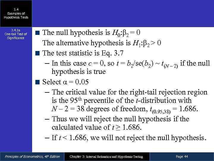3. 4 Examples of Hypothesis Tests 3. 4. 1 a One-tail Test of Significance The null hypothesis is H 0: β 2 = 0 The alternative hypothesis is H 1: β 2 > 0 The test statistic is Eq. 3. 7 – In this case c = 0, so t = b 2/se(b 2) ~ t(N – 2) if the null hypothesis is true Select α = 0. 05 – The critical value for the right-tail rejection region is the 95 th percentile of the t-distribution with N – 2 = 38 degrees of freedom, t(0. 95, 38) = 1. 686. – Thus we will reject the null hypothesis if the calculated value of t ≥ 1. 686. – If t < 1. 686, we will not reject the null hypothesis. Principles of Econometrics, 4 th Edition Chapter 3: Interval Estimation and Hypothesis Testing Page 44

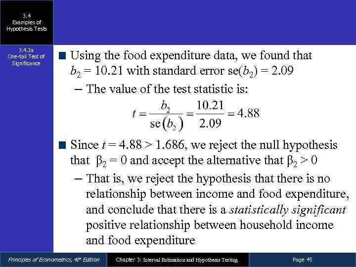3. 4 Examples of Hypothesis Tests 3. 4. 1 a One-tail Test of Significance Using the food expenditure data, we found that b 2 = 10. 21 with standard error se(b 2) = 2. 09 – The value of the test statistic is: Since t = 4. 88 > 1. 686, we reject the null hypothesis that β 2 = 0 and accept the alternative that β 2 > 0 – That is, we reject the hypothesis that there is no relationship between income and food expenditure, and conclude that there is a statistically significant positive relationship between household income and food expenditure Principles of Econometrics, 4 th Edition Chapter 3: Interval Estimation and Hypothesis Testing Page 45

3. 4 Examples of Hypothesis Tests 3. 4. 1 b One-tail Test of an Economic Hypothesis The null hypothesis is H 0: β 2 ≤ 5. 5 The alternative hypothesis is H 1: β 2 > 5. 5 The test statistic is t = (b 2 - 5. 5)/se(b 2) ~ t(N – 2) if the null hypothesis is true Select α = 0. 01 – The critical value for the right-tail rejection region is the 99 th percentile of the t-distribution with N – 2 = 38 degrees of freedom, t(0. 99, 38) = 2. 429 – Thus we will reject the null hypothesis if the calculated value of t ≥ 2. 429 – If t < 2. 429, we will not reject the null hypothesis Principles of Econometrics, 4 th Edition Chapter 3: Interval Estimation and Hypothesis Testing Page 46

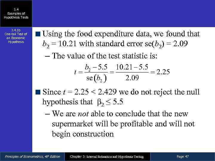3. 4 Examples of Hypothesis Tests 3. 4. 1 b One-tail Test of an Economic Hypothesis Using the food expenditure data, we found that b 2 = 10. 21 with standard error se(b 2) = 2. 09 – The value of the test statistic is: Since t = 2. 25 < 2. 429 we do not reject the null hypothesis that β 2 ≤ 5. 5 – We are not able to conclude that the new supermarket will be profitable and will not begin construction Principles of Econometrics, 4 th Edition Chapter 3: Interval Estimation and Hypothesis Testing Page 47

3. 4 Examples of Hypothesis Tests 3. 4. 2 Left-tail Tests The null hypothesis is H 0: β 2 ≥ 15 The alternative hypothesis is H 1: β 2 < 15 The test statistic is t = (b 2 - 15)/se(b 2) ~ t(N – 2) if the null hypothesis is true Select α = 0. 05 – The critical value for the left-tail rejection region is the 5 th percentile of the t-distribution with N – 2 = 38 degrees of freedom, t(0. 05, 38) = -1. 686. – Thus we will reject the null hypothesis if the calculated value of t ≤ -1. 686 – If t > -1. 686, we will not reject the null hypothesis Principles of Econometrics, 4 th Edition Chapter 3: Interval Estimation and Hypothesis Testing Page 48

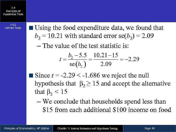3. 4 Examples of Hypothesis Tests 3. 4. 2 Left-tail Tests Using the food expenditure data, we found that b 2 = 10. 21 with standard error se(b 2) = 2. 09 – The value of the test statistic is: Since t = -2. 29 < -1. 686 we reject the null hypothesis that β 2 ≥ 15 and accept the alternative that β 2 < 15 – We conclude that households spend less than $15 from each additional $100 income on food Principles of Econometrics, 4 th Edition Chapter 3: Interval Estimation and Hypothesis Testing Page 49

3. 4 Examples of Hypothesis Tests 3. 4. 3 a Two-tail Test of an Economic Hypothesis The null hypothesis is H 0: β 2 = 7. 5 The alternative hypothesis is H 1: β 2 ≠ 7. 5 The test statistic is t = (b 2 – 7. 5)/se(b 2) ~ t(N – 2) if the null hypothesis is true Select α = 0. 05 – The critical value for the two-tail rejection region is the 2. 5 th percentile of the t-distribution with N – 2 = 38 degrees of freedom, t(0. 025, 38) = -2. 024 and the 97. 5 th percentile t(0. 975, 38) = 2. 024 – Thus we will reject the null hypothesis if the calculated value of t ≥ 2. 024 or if t ≤ -2. 024 Principles of Econometrics, 4 th Edition Chapter 3: Interval Estimation and Hypothesis Testing Page 50

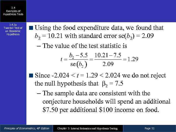3. 4 Examples of Hypothesis Tests 3. 4. 3 a Two-tail Test of an Economic Hypothesis Using the food expenditure data, we found that b 2 = 10. 21 with standard error se(b 2) = 2. 09 – The value of the test statistic is Since -2. 024 < t = 1. 29 < 2. 024 we do not reject the null hypothesis that β 2 = 7. 5 – The sample data are consistent with the conjecture households will spend an additional $7. 50 per additional $100 income on food. Principles of Econometrics, 4 th Edition Chapter 3: Interval Estimation and Hypothesis Testing Page 51

3. 4 Examples of Hypothesis Tests 3. 4. 3 b Two-tail Test of Significance The null hypothesis is H 0: β 2 = 0 The alternative hypothesis is H 1: β 2 ≠ 0 The test statistic is t = (b 2)/se(b 2) ~ t(N – 2) if the null hypothesis is true Select α = 0. 05 – The critical value for the two-tail rejection region is the 2. 5 th percentile of the t-distribution with N – 2 = 38 degrees of freedom, t(0. 025, 38) = -2. 024 and the 97. 5 th percentile t(0. 975, 38) = 2. 024 – Thus we will reject the null hypothesis if the calculated value of t ≥ 2. 024 or if t ≤ -2. 024 Principles of Econometrics, 4 th Edition Chapter 3: Interval Estimation and Hypothesis Testing Page 52

3. 4 Examples of Hypothesis Tests 3. 4. 3 b Two-tail Test of Significance Using the food expenditure data, we found that b 2 = 10. 21 with standard error se(b 2) = 2. 09 – The value of the test statistic is Since 4. 88 > 2. 024 we reject the null hypothesis that β 2 = 0 – We conclude that there is a statistically significant relationship between income and food expenditure Principles of Econometrics, 4 th Edition Chapter 3: Interval Estimation and Hypothesis Testing Page 53

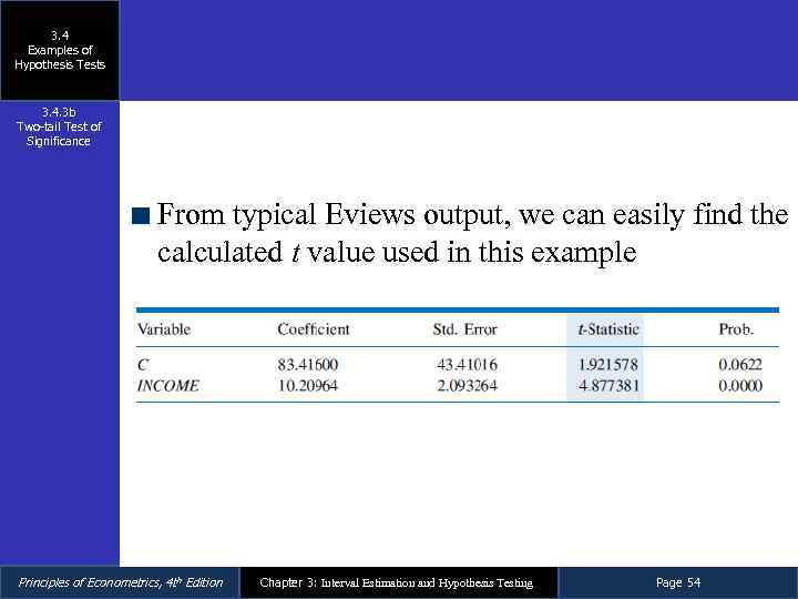3. 4 Examples of Hypothesis Tests 3. 4. 3 b Two-tail Test of Significance From typical Eviews output, we can easily find the calculated t value used in this example Principles of Econometrics, 4 th Edition Chapter 3: Interval Estimation and Hypothesis Testing Page 54

3. 5 The p-Value Principles of Econometrics, 4 th Edition Chapter 3: Interval Estimation and Hypothesis Testing Page 55

3. 5 The p-Value When reporting the outcome of statistical hypothesis tests, it has become standard practice to report the p-value (an abbreviation for probability value) of the test. – If we have the p-value of a test, p, we can determine the outcome of the test by comparing the p-value to the chosen level of significance, α, without looking up or calculating the critical values. • This is much more convenient Principles of Econometrics, 4 th Edition Chapter 3: Interval Estimation and Hypothesis Testing Page 56

3. 5 The p-Value p-VALUE RULE Reject the null hypothesis when the p-value is less than, or equal to, the level of significance α. That is, if p ≤ α then reject H 0. If p > α then do not reject H 0. Principles of Econometrics, 4 th Edition Chapter 3: Interval Estimation and Hypothesis Testing Page 57

3. 5 The p-Value If t is the calculated value of the t-statistic, then: – if H 1: βK > c p = probability to the right of t – if H 1: βK < c p = probability to the left of t – if H 1: βK ≠ c p = sum of probabilities to the right of |t| and to the left of – |t| Principles of Econometrics, 4 th Edition Chapter 3: Interval Estimation and Hypothesis Testing Page 58

3. 5 The p-Value 3. 5. 1 p-Value for a Right-tail Test From Section 3. 4. 1 b, we have – The null hypothesis is H 0: β 2 ≤ 5. 5 – The alternative hypothesis is H 1: β 2 > 5. 5 – The p-value is Principles of Econometrics, 4 th Edition Chapter 3: Interval Estimation and Hypothesis Testing Page 59

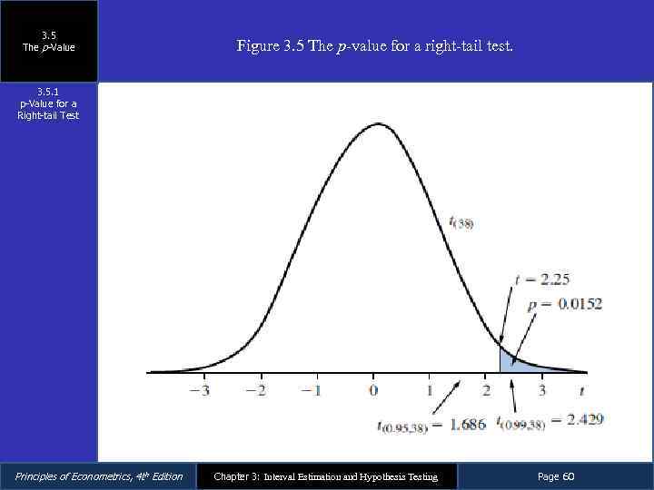3. 5 The p-Value Figure 3. 5 The p-value for a right-tail test. 3. 5. 1 p-Value for a Right-tail Test Principles of Econometrics, 4 th Edition Chapter 3: Interval Estimation and Hypothesis Testing Page 60

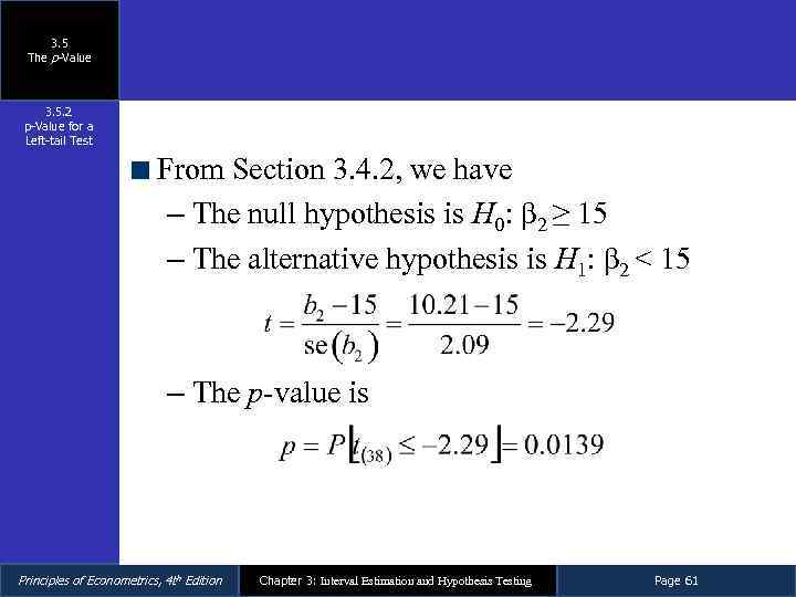3. 5 The p-Value 3. 5. 2 p-Value for a Left-tail Test From Section 3. 4. 2, we have – The null hypothesis is H 0: β 2 ≥ 15 – The alternative hypothesis is H 1: β 2 < 15 – The p-value is Principles of Econometrics, 4 th Edition Chapter 3: Interval Estimation and Hypothesis Testing Page 61

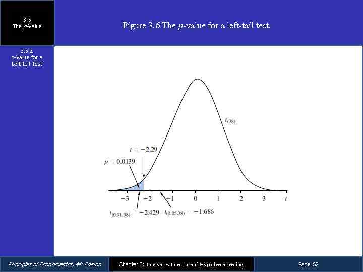3. 5 The p-Value Figure 3. 6 The p-value for a left-tail test. 3. 5. 2 p-Value for a Left-tail Test Principles of Econometrics, 4 th Edition Chapter 3: Interval Estimation and Hypothesis Testing Page 62

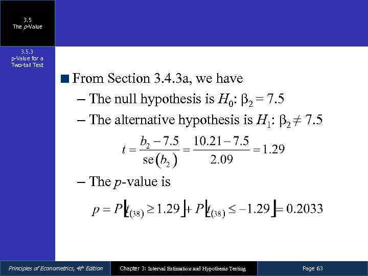3. 5 The p-Value 3. 5. 3 p-Value for a Two-tail Test From Section 3. 4. 3 a, we have – The null hypothesis is H 0: β 2 = 7. 5 – The alternative hypothesis is H 1: β 2 ≠ 7. 5 – The p-value is Principles of Econometrics, 4 th Edition Chapter 3: Interval Estimation and Hypothesis Testing Page 63

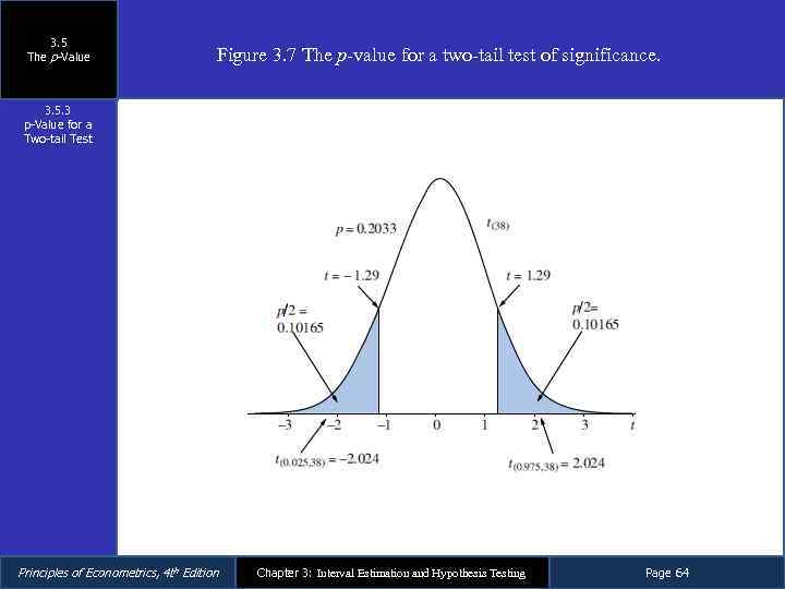3. 5 The p-Value Figure 3. 7 The p-value for a two-tail test of significance. 3. 5. 3 p-Value for a Two-tail Test Principles of Econometrics, 4 th Edition Chapter 3: Interval Estimation and Hypothesis Testing Page 64

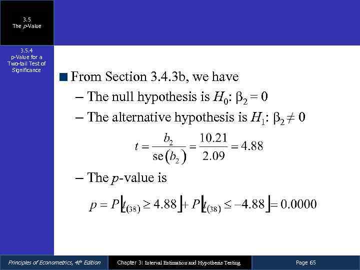3. 5 The p-Value 3. 5. 4 p-Value for a Two-tail Test of Significance From Section 3. 4. 3 b, we have – The null hypothesis is H 0: β 2 = 0 – The alternative hypothesis is H 1: β 2 ≠ 0 – The p-value is Principles of Econometrics, 4 th Edition Chapter 3: Interval Estimation and Hypothesis Testing Page 65

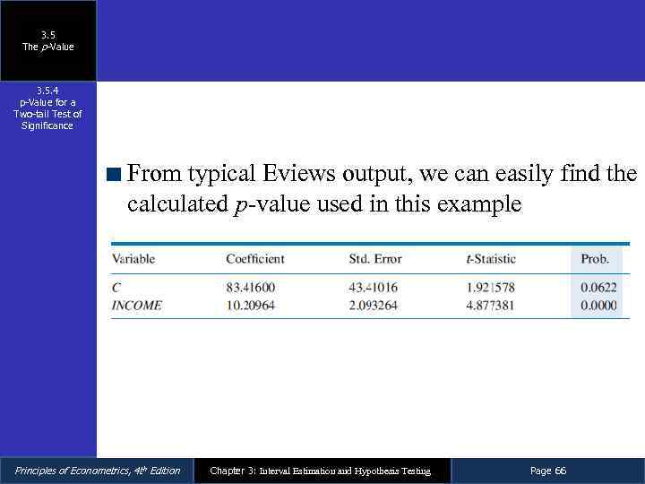3. 5 The p-Value 3. 5. 4 p-Value for a Two-tail Test of Significance From typical Eviews output, we can easily find the calculated p-value used in this example Principles of Econometrics, 4 th Edition Chapter 3: Interval Estimation and Hypothesis Testing Page 66

3. 6 Linear Combinations of Parameters Principles of Econometrics, 4 th Edition Chapter 3: Interval Estimation and Hypothesis Testing Page 67

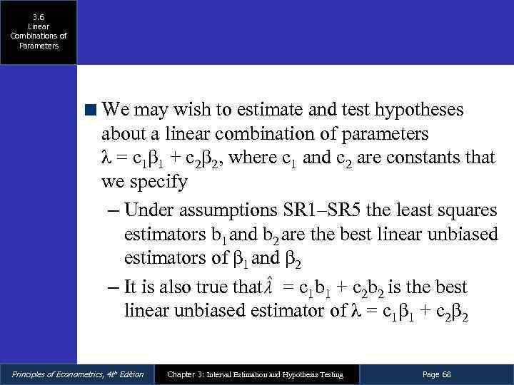3. 6 Linear Combinations of Parameters We may wish to estimate and test hypotheses about a linear combination of parameters λ = c 1β 1 + c 2β 2, where c 1 and c 2 are constants that we specify – Under assumptions SR 1–SR 5 the least squares estimators b 1 and b 2 are the best linear unbiased estimators of β 1 and β 2 – It is also true that = c 1 b 1 + c 2 b 2 is the best linear unbiased estimator of λ = c 1β 1 + c 2β 2 Principles of Econometrics, 4 th Edition Chapter 3: Interval Estimation and Hypothesis Testing Page 68

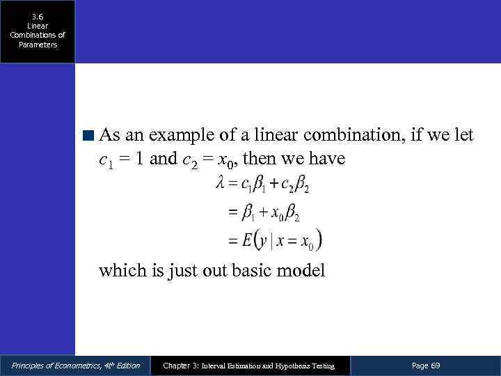3. 6 Linear Combinations of Parameters As an example of a linear combination, if we let c 1 = 1 and c 2 = x 0, then we have which is just out basic model Principles of Econometrics, 4 th Edition Chapter 3: Interval Estimation and Hypothesis Testing Page 69

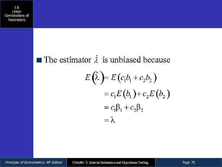3. 6 Linear Combinations of Parameters The estimator Principles of Econometrics, 4 th Edition is unbiased because Chapter 3: Interval Estimation and Hypothesis Testing Page 70

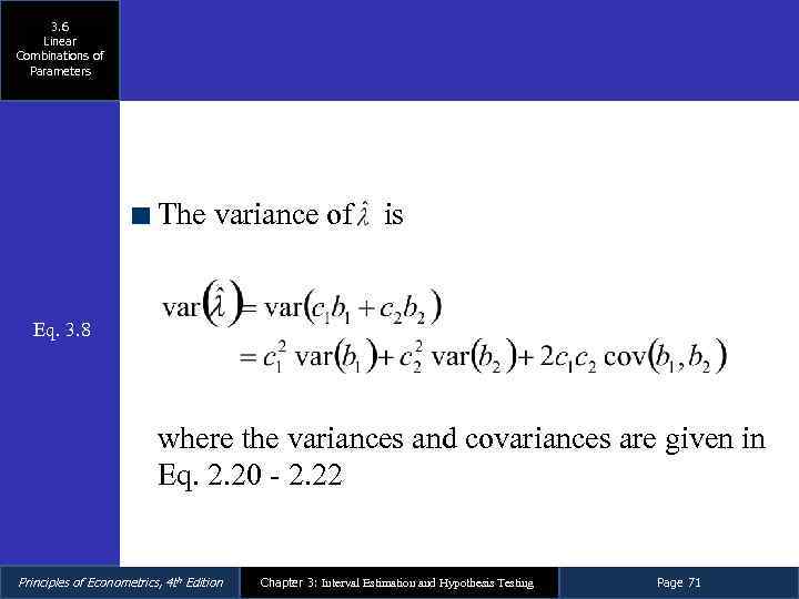3. 6 Linear Combinations of Parameters The variance of is Eq. 3. 8 where the variances and covariances are given in Eq. 2. 20 - 2. 22 Principles of Econometrics, 4 th Edition Chapter 3: Interval Estimation and Hypothesis Testing Page 71

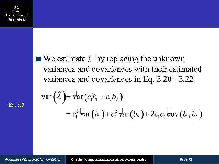3. 6 Linear Combinations of Parameters We estimate by replacing the unknown variances and covariances with their estimated variances and covariances in Eq. 2. 20 - 2. 22 Eq. 3. 9 Principles of Econometrics, 4 th Edition Chapter 3: Interval Estimation and Hypothesis Testing Page 72

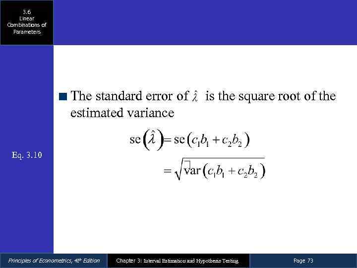3. 6 Linear Combinations of Parameters The standard error of estimated variance is the square root of the Eq. 3. 10 Principles of Econometrics, 4 th Edition Chapter 3: Interval Estimation and Hypothesis Testing Page 73

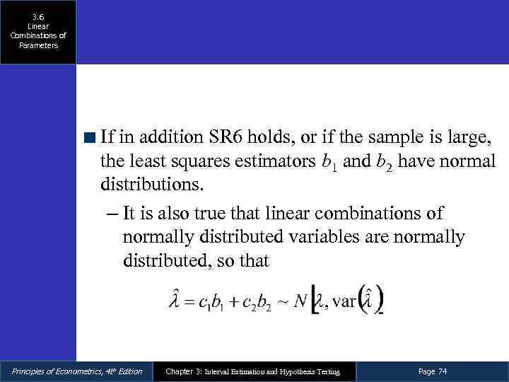3. 6 Linear Combinations of Parameters If in addition SR 6 holds, or if the sample is large, the least squares estimators b 1 and b 2 have normal distributions. – It is also true that linear combinations of normally distributed variables are normally distributed, so that Principles of Econometrics, 4 th Edition Chapter 3: Interval Estimation and Hypothesis Testing Page 74

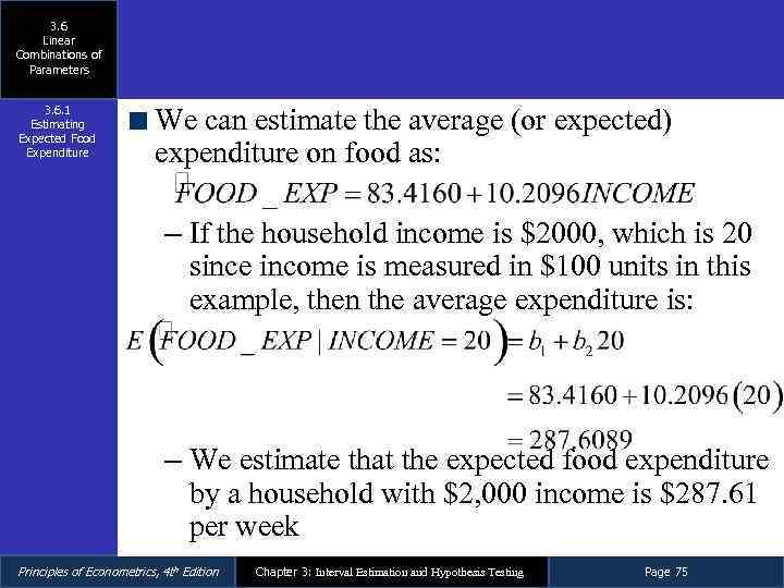3. 6 Linear Combinations of Parameters 3. 6. 1 Estimating Expected Food Expenditure We can estimate the average (or expected) expenditure on food as: – If the household income is $2000, which is 20 since income is measured in $100 units in this example, then the average expenditure is: – We estimate that the expected food expenditure by a household with $2, 000 income is $287. 61 per week Principles of Econometrics, 4 th Edition Chapter 3: Interval Estimation and Hypothesis Testing Page 75

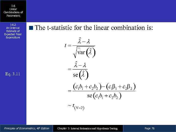3. 6 Linear Combinations of Parameters 3. 6. 2 An Interval Estimate of Expected Food Expenditure The t-statistic for the linear combination is: Eq. 3. 11 Principles of Econometrics, 4 th Edition Chapter 3: Interval Estimation and Hypothesis Testing Page 76

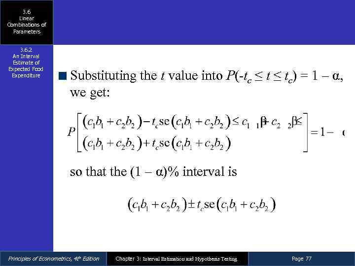3. 6 Linear Combinations of Parameters 3. 6. 2 An Interval Estimate of Expected Food Expenditure Substituting the t value into P(-tc ≤ tc) = 1 – α, we get: so that the (1 – α)% interval is Principles of Econometrics, 4 th Edition Chapter 3: Interval Estimation and Hypothesis Testing Page 77

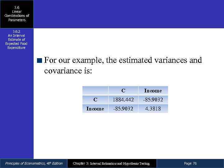3. 6 Linear Combinations of Parameters 3. 6. 2 An Interval Estimate of Expected Food Expenditure For our example, the estimated variances and covariance is: C C 1884. 442 -85. 9032 Income Principles of Econometrics, 4 th Edition Income -85. 9032 4. 3818 Chapter 3: Interval Estimation and Hypothesis Testing Page 78

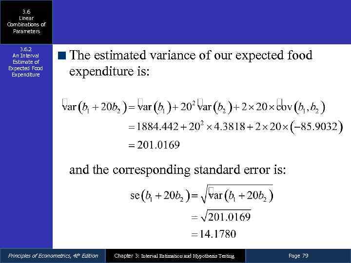3. 6 Linear Combinations of Parameters 3. 6. 2 An Interval Estimate of Expected Food Expenditure The estimated variance of our expected food expenditure is: and the corresponding standard error is: Principles of Econometrics, 4 th Edition Chapter 3: Interval Estimation and Hypothesis Testing Page 79

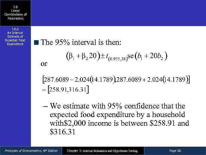3. 6 Linear Combinations of Parameters 3. 6. 2 An Interval Estimate of Expected Food Expenditure The 95% interval is then: or – We estimate with 95% confidence that the expected food expenditure by a household with$2, 000 income is between $258. 91 and $316. 31 Principles of Econometrics, 4 th Edition Chapter 3: Interval Estimation and Hypothesis Testing Page 80

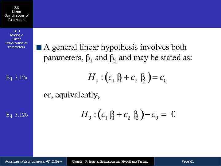3. 6 Linear Combinations of Parameters 3. 6. 3 Testing a Linear Combination of Parameters A general linear hypothesis involves both parameters, β 1 and β 2 and may be stated as: Eq. 3. 12 a or, equivalently, Eq. 3. 12 b Principles of Econometrics, 4 th Edition Chapter 3: Interval Estimation and Hypothesis Testing Page 81

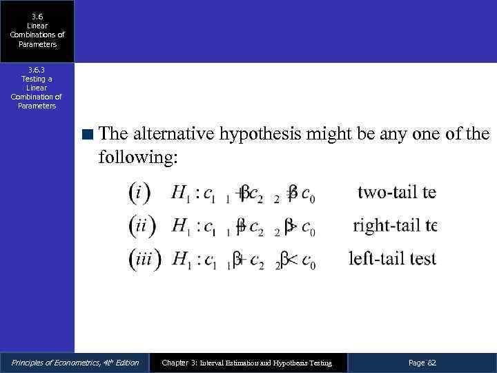3. 6 Linear Combinations of Parameters 3. 6. 3 Testing a Linear Combination of Parameters The alternative hypothesis might be any one of the following: Principles of Econometrics, 4 th Edition Chapter 3: Interval Estimation and Hypothesis Testing Page 82

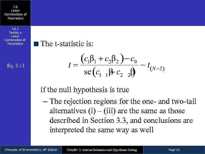3. 6 Linear Combinations of Parameters 3. 6. 3 Testing a Linear Combination of Parameters The t-statistic is: Eq. 3. 13 if the null hypothesis is true – The rejection regions for the one- and two-tail alternatives (i) – (iii) are the same as those described in Section 3. 3, and conclusions are interpreted the same way as well Principles of Econometrics, 4 th Edition Chapter 3: Interval Estimation and Hypothesis Testing Page 83

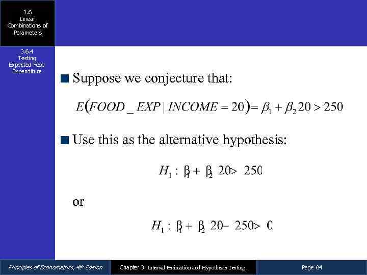3. 6 Linear Combinations of Parameters 3. 6. 4 Testing Expected Food Expenditure Suppose we conjecture that: Use this as the alternative hypothesis: or Principles of Econometrics, 4 th Edition Chapter 3: Interval Estimation and Hypothesis Testing Page 84

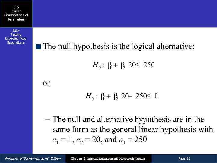3. 6 Linear Combinations of Parameters 3. 6. 4 Testing Expected Food Expenditure The null hypothesis is the logical alternative: or – The null and alternative hypothesis are in the same form as the general linear hypothesis with c 1 = 1, c 2 = 20, and c 0 = 250 Principles of Econometrics, 4 th Edition Chapter 3: Interval Estimation and Hypothesis Testing Page 85

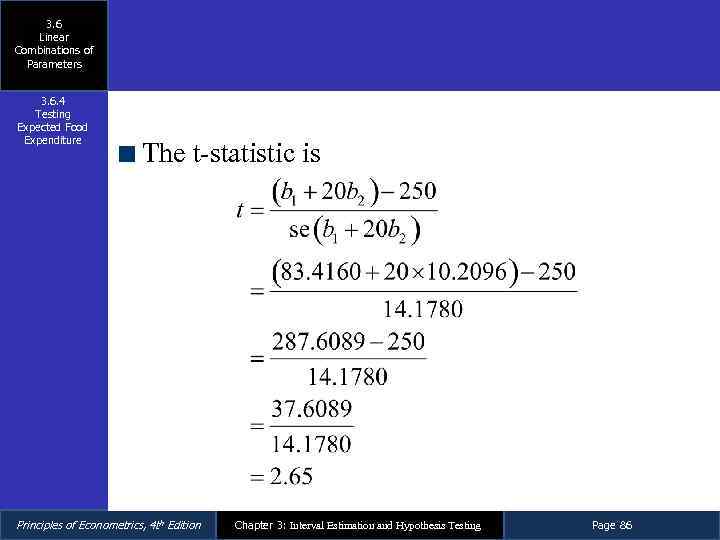3. 6 Linear Combinations of Parameters 3. 6. 4 Testing Expected Food Expenditure The t-statistic is Principles of Econometrics, 4 th Edition Chapter 3: Interval Estimation and Hypothesis Testing Page 86

3. 6 Linear Combinations of Parameters 3. 6. 4 Testing Expected Food Expenditure Since t =2. 65 > tc = 1. 686, we reject the null hypothesis that a household with weekly income of $2, 000 will spend $250 per week or less on food, and conclude that the conjecture that such households spend more than $250 is correct, with the probability of Type I error 0. 05 Principles of Econometrics, 4 th Edition Chapter 3: Interval Estimation and Hypothesis Testing Page 87

Key Words Principles of Econometrics, 4 th Edition Chapter 3: Interval Estimation and Hypothesis Testing Page 88

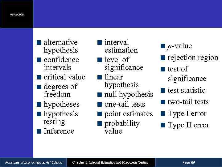Keywords alternative hypothesis confidence intervals critical value degrees of freedom hypotheses hypothesis testing Inference Principles of Econometrics, 4 th Edition interval estimation level of significance linear hypothesis null hypothesis one-tail tests point estimates probability value Chapter 3: Interval Estimation and Hypothesis Testing p-value rejection region test of significance test statistic two-tail tests Type I error Type II error Page 89

Appendices Principles of Econometrics, 4 th Edition Chapter 3: Interval Estimation and Hypothesis Testing Page 90

3 A Derivation of the t-distribution 3 B Distribution of the t-statistic under H 1 3 C Monte Carlo Simulation Principles of Econometrics, 4 th Edition Chapter 3: Interval Estimation and Hypothesis Testing Page 91

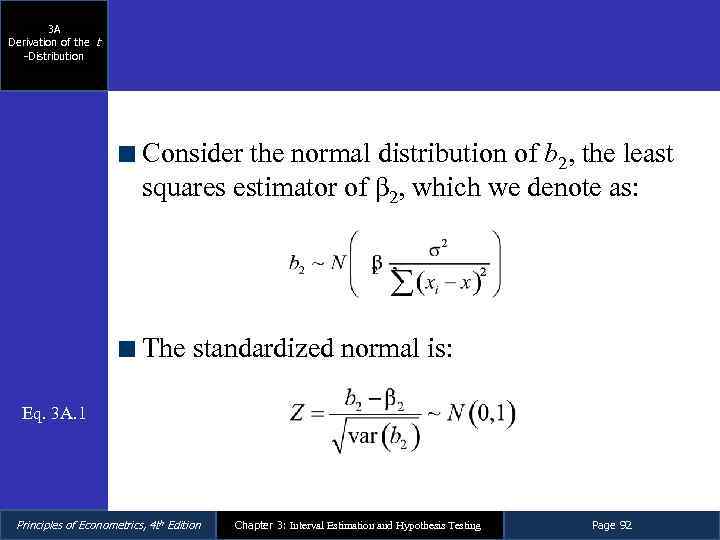3 A Derivation of the t -Distribution Consider the normal distribution of b 2, the least squares estimator of β 2, which we denote as: The standardized normal is: Eq. 3 A. 1 Principles of Econometrics, 4 th Edition Chapter 3: Interval Estimation and Hypothesis Testing Page 92

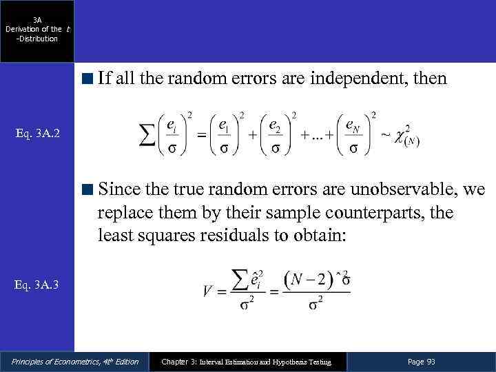3 A Derivation of the t -Distribution If all the random errors are independent, then Eq. 3 A. 2 Since the true random errors are unobservable, we replace them by their sample counterparts, the least squares residuals to obtain: Eq. 3 A. 3 Principles of Econometrics, 4 th Edition Chapter 3: Interval Estimation and Hypothesis Testing Page 93

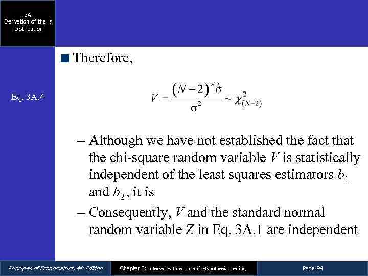3 A Derivation of the t -Distribution Therefore, Eq. 3 A. 4 – Although we have not established the fact that the chi-square random variable V is statistically independent of the least squares estimators b 1 and b 2 , it is – Consequently, V and the standard normal random variable Z in Eq. 3 A. 1 are independent Principles of Econometrics, 4 th Edition Chapter 3: Interval Estimation and Hypothesis Testing Page 94

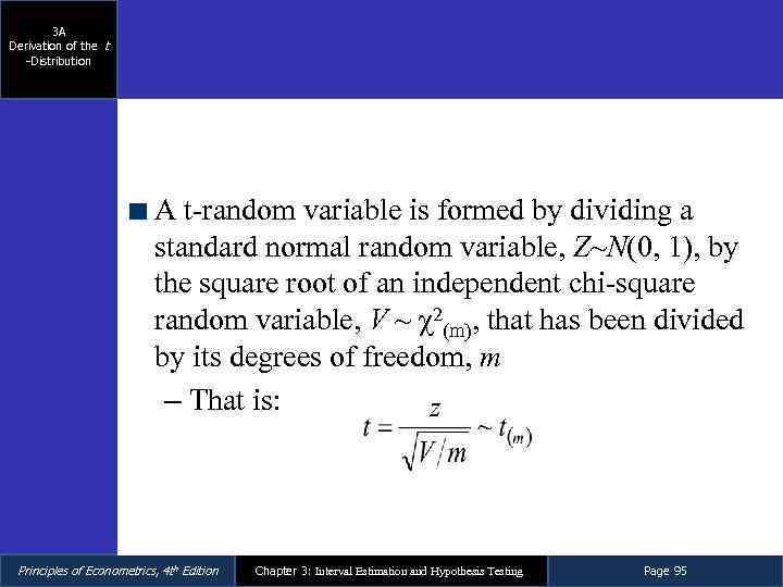3 A Derivation of the t -Distribution A t-random variable is formed by dividing a standard normal random variable, Z~N(0, 1), by the square root of an independent chi-square random variable, V ~ χ2(m), that has been divided by its degrees of freedom, m – That is: Principles of Econometrics, 4 th Edition Chapter 3: Interval Estimation and Hypothesis Testing Page 95

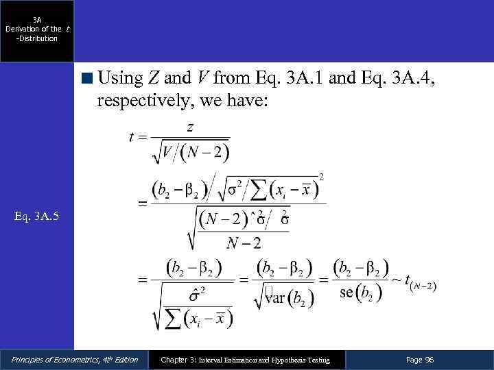3 A Derivation of the t -Distribution Using Z and V from Eq. 3 A. 1 and Eq. 3 A. 4, respectively, we have: Eq. 3 A. 5 Principles of Econometrics, 4 th Edition Chapter 3: Interval Estimation and Hypothesis Testing Page 96

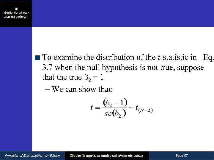3 B Distribution of the t. Statistic under H 1 To examine the distribution of the t-statistic in Eq. 3. 7 when the null hypothesis is not true, suppose that the true β 2 = 1 – We can show that: Principles of Econometrics, 4 th Edition Chapter 3: Interval Estimation and Hypothesis Testing Page 97

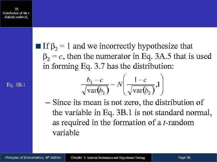3 B Distribution of the t. Statistic under H 1 If β 2 = 1 and we incorrectly hypothesize that β 2 = c, then the numerator in Eq. 3 A. 5 that is used in forming Eq. 3. 7 has the distribution: Eq. 3 B. 1 – Since its mean is not zero, the distribution of the variable in Eq. 3 B. 1 is not standard normal, as required in the formation of a t-random variable Principles of Econometrics, 4 th Edition Chapter 3: Interval Estimation and Hypothesis Testing Page 98

3 C Monte Carlo Simulation When studying the performance of hypothesis tests and interval estimators it is necessary to use enough Monte Carlo samples so that the percentages involved are estimated precisely enough to be useful – For tests with probability of Type I error α = 0. 05 we should observe true null hypotheses being rejected 5% of the time – For 95% interval estimators we should observe that 95% of the interval estimates contain the true parameter values – We use M = 10, 000 Monte Carlo samples so that the experimental error is very small Principles of Econometrics, 4 th Edition Chapter 3: Interval Estimation and Hypothesis Testing Page 99

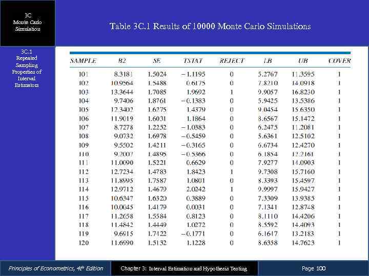3 C Monte Carlo Simulation Table 3 C. 1 Results of 10000 Monte Carlo Simulations 3 C. 1 Repeated Sampling Properties of Interval Estimators Principles of Econometrics, 4 th Edition Chapter 3: Interval Estimation and Hypothesis Testing Page 100

3 C Monte Carlo Simulation 3 C. 1 Repeated Sampling Properties of Interval Estimators The lesson is, that in many repeated samples from the data generation process, and if assumptions SR 1–SR 6 hold, the procedure for constructing 95% interval estimates ‘‘works’’ 95% of the time Principles of Econometrics, 4 th Edition Chapter 3: Interval Estimation and Hypothesis Testing Page 101

3 C Monte Carlo Simulation 3 C. 2 Repeated Sampling Properties of Hypothesis Tests The lesson is that in many repeated samples from the data generation process, and if assumptions SR 1–SR 6 hold, the procedure for testing a true null hypothesis at significance level α = 0. 05 rejects the true null hypothesis 5% of the time – Or, stated positively, the test procedure does not reject the true null hypothesis 95% of the time Principles of Econometrics, 4 th Edition Chapter 3: Interval Estimation and Hypothesis Testing Page 102

3 C Monte Carlo Simulation 3 C. 3 Choosing te Number of Monte Carlo Samples The point is that if fewer Monte Carlo samples are chosen the ‘‘noise’’ in the Monte Carlo experiment can lead to a percent of successes or rejections that has too wide a margin of error for us to tell whether the statistical procedure, interval estimation, or hypothesis testing, is ‘‘working’’ properly or not Principles of Econometrics, 4 th Edition Chapter 3: Interval Estimation and Hypothesis Testing Page 103