Chapter 3 Forecasting 1 Forecast OM

Chapter 3 Forecasting 1

Forecast • OM is mostly proactive not reactive • It involves structured planning activities • Planning requires data pertaining to the feature • Forecast: A statement about the future – Not necessarily numerical • Weather forecasts 2

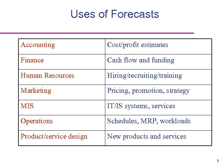Uses of Forecasts Accounting Cost/profit estimates Finance Cash flow and funding Human Resources Hiring/recruiting/training Marketing Pricing, promotion, strategy MIS IT/IS systems, services Operations Schedules, MRP, workloads Product/service design New products and services 3

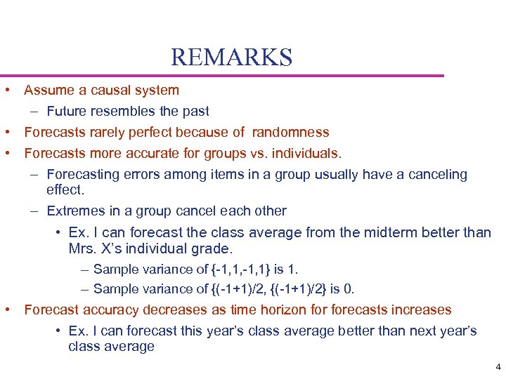REMARKS • Assume a causal system – Future resembles the past • Forecasts rarely perfect because of randomness • Forecasts more accurate for groups vs. individuals. – Forecasting errors among items in a group usually have a canceling effect. – Extremes in a group cancel each other • Ex. I can forecast the class average from the midterm better than Mrs. X’s individual grade. – Sample variance of {-1, 1, -1, 1} is 1. – Sample variance of {(-1+1)/2, {(-1+1)/2} is 0. • Forecast accuracy decreases as time horizon forecasts increases • Ex. I can forecast this year’s class average better than next year’s class average 4

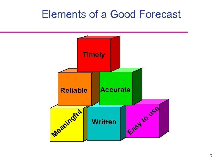Elements of a Good Forecast Timely Reliable ul M e gf n ni a Accurate Written sy Ea to se u 5

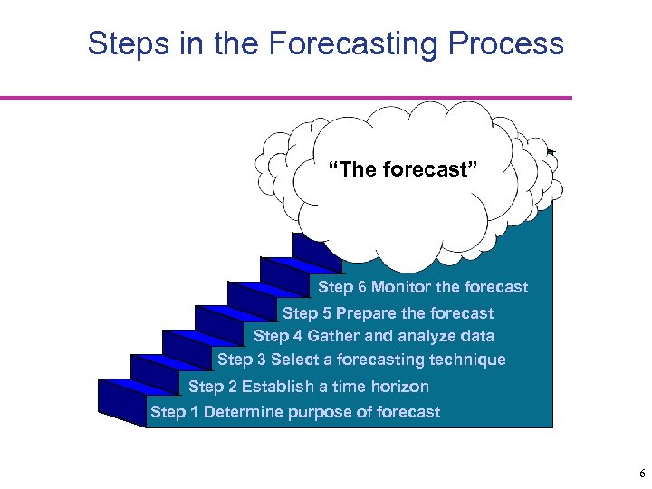Steps in the Forecasting Process “The forecast” Step 6 Monitor the forecast Step 5 Prepare the forecast Step 4 Gather and analyze data Step 3 Select a forecasting technique Step 2 Establish a time horizon Step 1 Determine purpose of forecast 6

Types of Forecasts • Judgmental - Subjective analysis of subjective inputs • Associative models – Analyzes historical data to reveal relationships between (easily or in advance) observable quantities and forecast quantities. Uses this relationship to make predictions. • Time series – Objective analysis historical data assuming the future will be like the past 7

Judgmental Forecasts • Executive opinions (long-range planning) – There are factors hard to quantify • Ex: Effects of November 2004 election on new houses built in 2005 • Sales force composite – Retailer forecasts for the manufacturer • Consumer surveys – The guy at the mall who asks if you like cherry flavor in your shampoo • Outside opinion – Financial and consulting gurus and companies • Opinions of managers and staff – Delphi method: A series of questionnaires developed sequentially 8

Associative Forecasting • Based on identification of related variables that can be used to predict values of the variable of interest. – Sales of mountain bikes in an area may be related to the percentage of the young population living in that area. – Sales of Harley-Davidson motorbikes is related to mid-aged men population. Average of H-D owners is 46. – Ice cream sales can be related to temperature – Home depot bases sales forecasts on mortgage refinancing rates, smaller rates imply higher sales. – Changes in Federal Reserve Board’s interest rate leads to certain business activities • House sales • Industrial investments – Increase in energy cost leads to price increases in products and services 9

Associative Forecasting • Find an association between the predictor and the predicted • Predictor variables - used to predict values of variable interest, sometimes called independent variables • Predicted variable = Dependent variable • Regression - technique for fitting a line to a set of points • Linear regression is the most widely used form of regression – The objective is to obtain an equation of a straight line that minimizes the sum of squared vertical deviations of data points from the line. 10

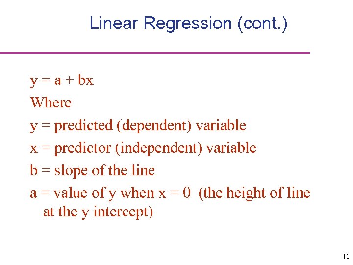Linear Regression (cont. ) y = a + bx Where y = predicted (dependent) variable x = predictor (independent) variable b = slope of the line a = value of y when x = 0 (the height of line at the y intercept) 11

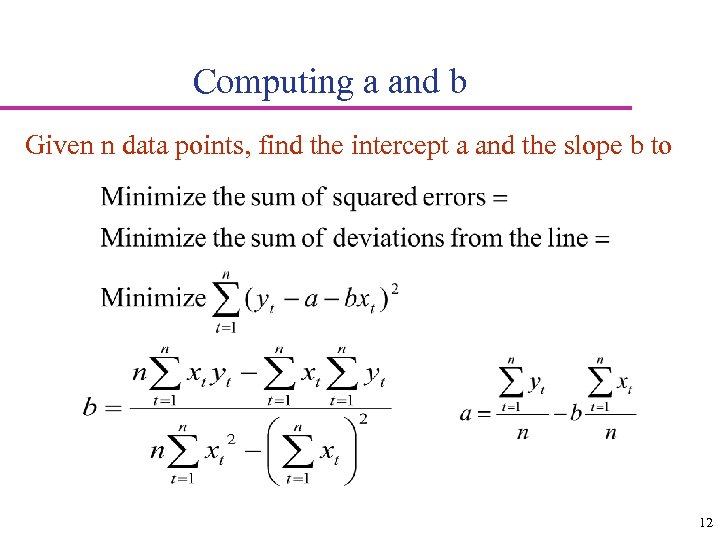Computing a and b Given n data points, find the intercept a and the slope b to 12

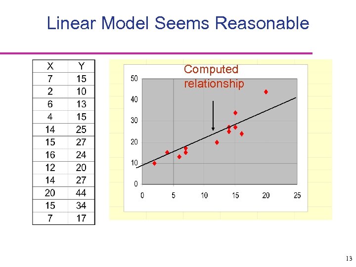Linear Model Seems Reasonable Computed relationship 13

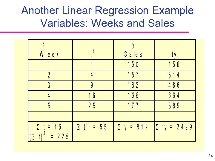Another Linear Regression Example Variables: Weeks and Sales 14

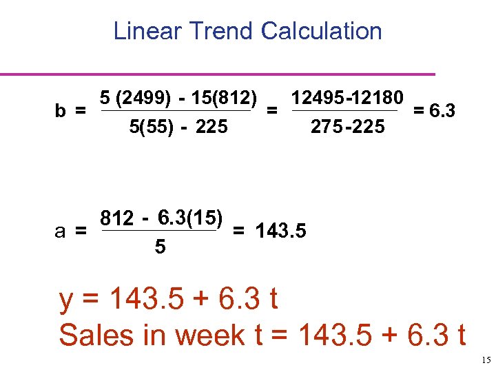Linear Trend Calculation 5 (2499) - 15(812) 12495 -12180 b = = = 6. 3 5(55) - 225 275 -225 812 - 6. 3(15) a = = 143. 5 5 y = 143. 5 + 6. 3 t Sales in week t = 143. 5 + 6. 3 t 15

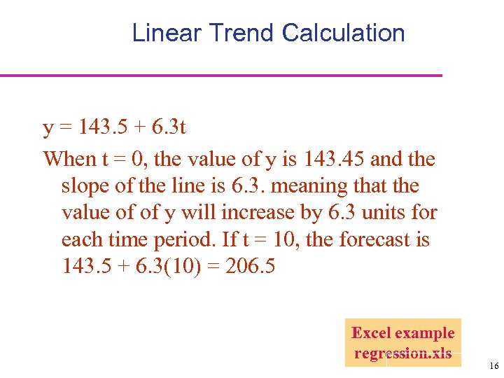Linear Trend Calculation y = 143. 5 + 6. 3 t When t = 0, the value of y is 143. 45 and the slope of the line is 6. 3. meaning that the value of of y will increase by 6. 3 units for each time period. If t = 10, the forecast is 143. 5 + 6. 3(10) = 206. 5 Excel example regression. xls 16

Linear Regression Remember from Statistics • Correlation (r) between variables: The strength and direction of relationships between two variables – 1. 00 means changes in one variable are always matched by changes in the other, vice versa. – A correlation close to zero means little linear relationship – The square of the correlation coefficient provides a measure of the percentage of variability in the values of y that is explained by the independent variable. (80% or more: the independent variable is a good predictor of the values of dependent variable) 17

Time series • Time-ordered sequence of observations taken at regular intervals over a period of time • Future values of the series can be estimated from past values. Types of Variations in Time Series Data • • • Trend - long-term movement in data Seasonality - short-term regular variations in data Cycles – wavelike variations of long-term Irregular variations - caused by unusual circumstances Random variations - caused by chance 18

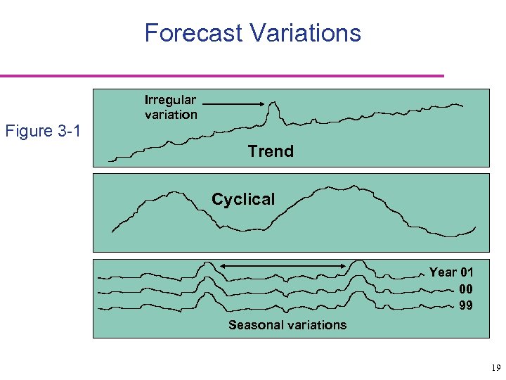Forecast Variations Figure 3 -1 Irregular variation Trend Cyclical Cycles Year 01 00 99 Seasonal variations 19

Naïve Forecasts • Uses a single previous value of a time series as the basis of a forecast. • Virtually no cost • Data analysis is nonexistent • Easily understandable • Cannot provide high accuracy – If it were true, future will always be the same as the past Some notation: Forecast at time t is F(t) Actual observation at time t is A(t) Today is temperature is 98 F, A(Today)=98 F(Tomorrow)=98 F(Day after)=98 20

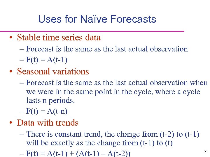Uses for Naïve Forecasts • Stable time series data – Forecast is the same as the last actual observation – F(t) = A(t-1) • Seasonal variations – Forecast is the same as the last actual observation when we were in the same point in the cycle, where a cycle lasts n periods. – F(t) = A(t-n) • Data with trends – There is constant trend, the change from (t-2) to (t-1) will be exactly as the change from (t-1) to (t) – F(t) = A(t-1) + (A(t-1) – A(t-2)) 21

Naive Forecasts Uh, give me a minute. . We sold 250 wheels last week. . Now, next week we should sell. . 22

Naïve (Cont. ) • Check if the resulting accuracy is acceptable • The higher the accuracy, often the higher the cost. • Do we really need our forecast that accurate? Is it worth the additional resources? – Why do you need forecasts for? How critical they are for operations? 23

Time Series Models: Variations What is random and what is not? • Historical data contain random variations or noise • Random variations are caused by relatively unimportant factors. – What is random? Can we not study everything to negligible detail? “God does not roll dices” –A. E. • The objective is to remove all randomness and have real variations. • Minor variations are random and large ones are real. 24

Techniques for Averaging • Moving averages (MA) – Naïve methods just trace the actual data with a lag of one period, F(t)=A(t-1) – They don’t smooth – MA uses a number of the most recent actual data to smooth • Weighted moving averages • Exponential smoothing 25

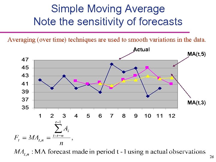Simple Moving Average Note the sensitivity of forecasts Averaging (over time) techniques are used to smooth variations in the data. Actual MA(t, 5) MA(t, 3) 26

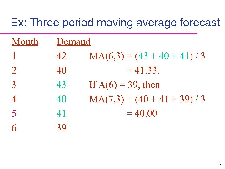Ex: Three period moving average forecast Month 1 2 3 4 5 6 Demand 42 MA(6, 3) = (43 + 40 + 41) / 3 40 = 41. 33. 43 If A(6) = 39, then 40 MA(7, 3) = (40 + 41 + 39) / 3 41 = 40. 00 39 27

Weighted average Moving Average • Advantage=Easy to compute and easy to understand • Disadvantage=All values in the average are weighted equally Weighted Moving Average • Similar to moving average • It assigns more weight to the most recent values in a time series – Idea: most recent observations must be better indicators of the future than older observations 28

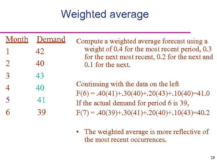Weighted average Month 1 2 3 4 5 6 Demand 42 40 43 40 41 39 Compute a weighted average forecast using a weight of 0. 4 for the most recent period, 0. 3 for the next most recent, 0. 2 for the next and 0. 1 for the next. Continuing with the data on the left F(6) =. 40(41)+. 30(40)+. 20(43)+. 10(40)=41. 0 If the actual demand for period 6 is 39, F(7) =. 40(39)+. 30(41)+. 20(40)+. 10(43)=40. 2 • The weighted average is more reflective of the most recent occurrences. 29

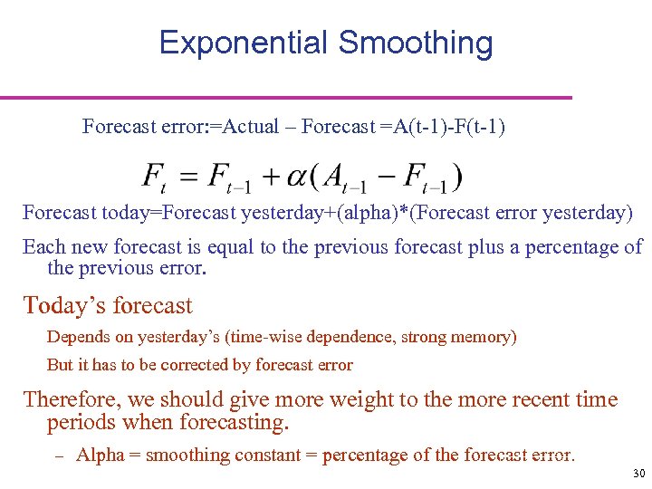Exponential Smoothing Forecast error: =Actual – Forecast =A(t-1)-F(t-1) Forecast today=Forecast yesterday+(alpha)*(Forecast error yesterday) Each new forecast is equal to the previous forecast plus a percentage of the previous error. Today’s forecast Depends on yesterday’s (time-wise dependence, strong memory) But it has to be corrected by forecast error Therefore, we should give more weight to the more recent time periods when forecasting. – Alpha = smoothing constant = percentage of the forecast error. 30

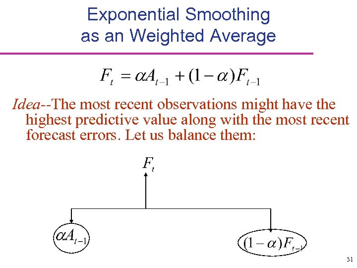Exponential Smoothing as an Weighted Average Idea--The most recent observations might have the highest predictive value along with the most recent forecast errors. Let us balance them: 31

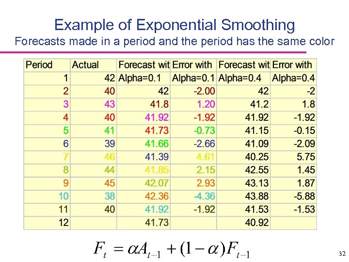Example of Exponential Smoothing Forecasts made in a period and the period has the same color 32

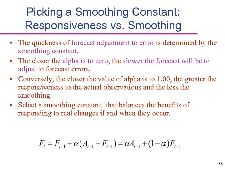Picking a Smoothing Constant: Responsiveness vs. Smoothing • The quickness of forecast adjustment to error is determined by the smoothing constant. • The closer the alpha is to zero, the slower the forecast will be to adjust to forecast errors. • Conversely, the closer the value of alpha is to 1. 00, the greater the responsiveness to the actual observations and the less the smoothing • Select a smoothing constant that balances the benefits of responding to real changes if and when they occur. 33

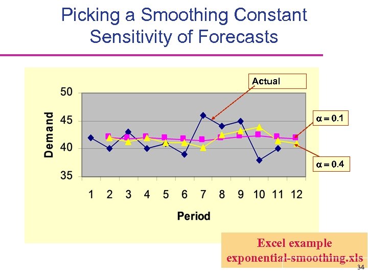Picking a Smoothing Constant Sensitivity of Forecasts Actual 0. 1 0. 4 Excel example exponential-smoothing. xls 34

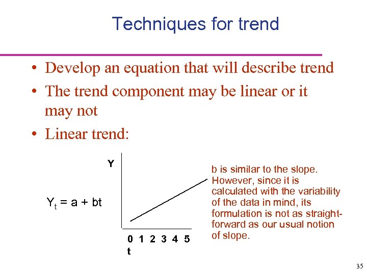Techniques for trend • Develop an equation that will describe trend • The trend component may be linear or it may not • Linear trend: Y Yt = a + bt 0 1 2 3 4 5 t b is similar to the slope. However, since it is calculated with the variability of the data in mind, its formulation is not as straightforward as our usual notion of slope. 35

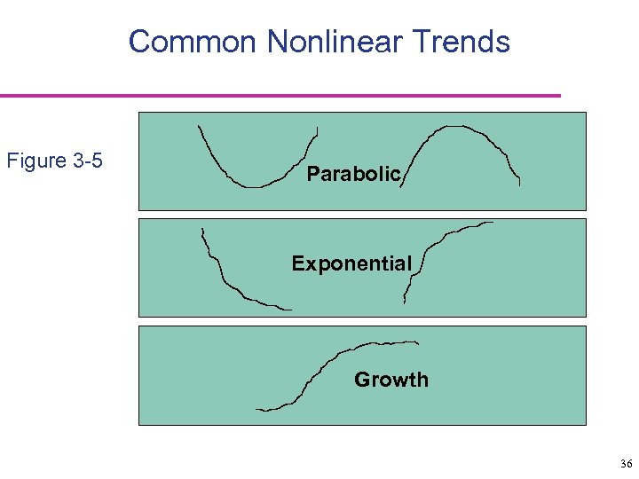Common Nonlinear Trends Figure 3 -5 Parabolic Exponential Growth 36

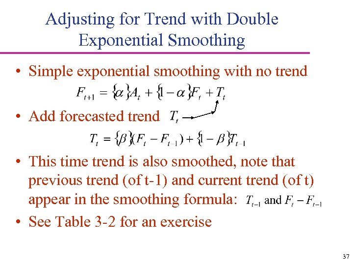Adjusting for Trend with Double Exponential Smoothing • Simple exponential smoothing with no trend • Add forecasted trend • This time trend is also smoothed, note that previous trend (of t-1) and current trend (of t) appear in the smoothing formula: • See Table 3 -2 for an exercise 37

Techniques for seasonality • Regularly repeating upward or downward movements in time series values • Seasonality: weather variations, vacations and holidays • Seasonality: Expressed in terms of the amount that actual values deviate from the average value of the series • Seasonality is expressed as a percentage of the average amount seasonal percentages = seasonal relatives = seasonal indices 38

Different models of seasonality – Seasonal relative = 1. 45 for the quantity of television sold in August at Circuit City, meaning that TV sales for that month are 45% above the monthly average. – Seasonal factor=0. 60 for the number of notebooks sold at the UTD bookstore in April, meaning that notebook sales are 40% below the monthly average. – Seasonal indices are your vehicle to travel between the seasonal and deseasonal worlds. 39

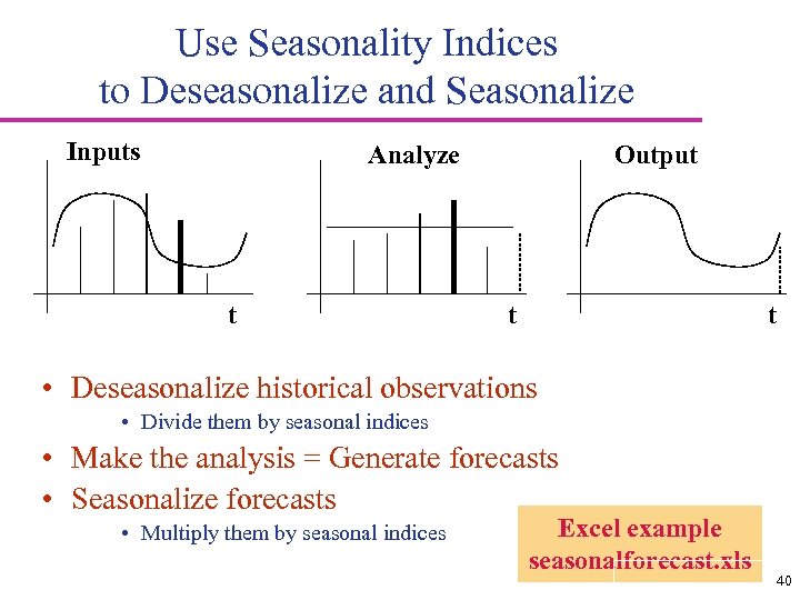Use Seasonality Indices to Deseasonalize and Seasonalize Inputs Analyze t Output t t • Deseasonalize historical observations • Divide them by seasonal indices • Make the analysis = Generate forecasts • Seasonalize forecasts • Multiply them by seasonal indices Excel example seasonalforecast. xls 40

Forecast Accuracy • Measurement is the first step to improve an activity – What value of smoothing constant is good? • Accuracy measurement is a vital aspect of forecasting • Impossible to correctly predict future values • Important to include an indication of how big the forecast deviate from the actual values 41

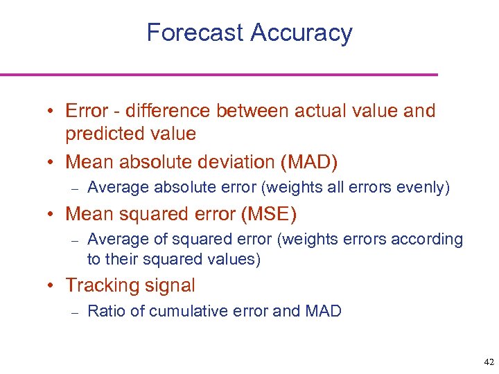Forecast Accuracy • Error - difference between actual value and predicted value • Mean absolute deviation (MAD) – Average absolute error (weights all errors evenly) • Mean squared error (MSE) – Average of squared error (weights errors according to their squared values) • Tracking signal – Ratio of cumulative error and MAD 42

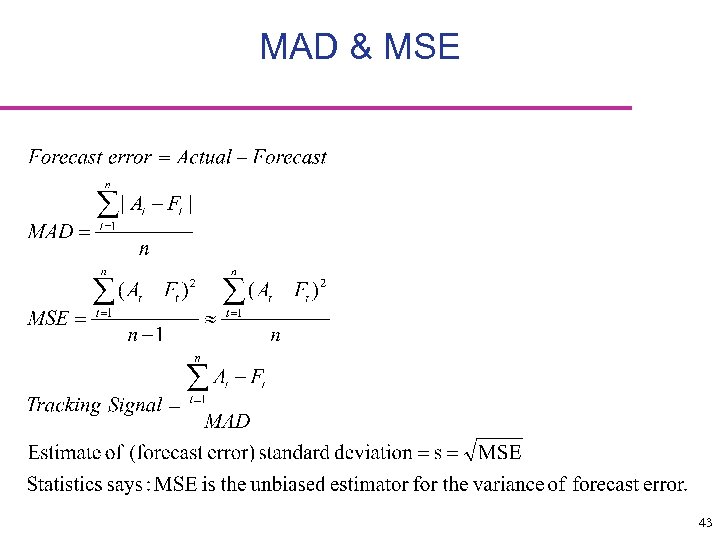MAD & MSE 43

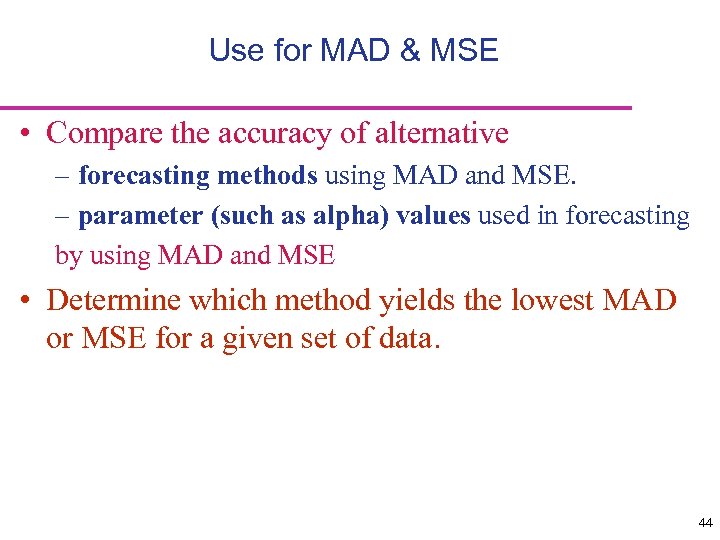Use for MAD & MSE • Compare the accuracy of alternative – forecasting methods using MAD and MSE. – parameter (such as alpha) values used in forecasting by using MAD and MSE • Determine which method yields the lowest MAD or MSE for a given set of data. 44

Controlling the quality of forecast • Necessary to monitor forecast to ensure that the forecast is performing adequately • This is accomplished by comparing forecast errors to predetermined values • Errors that fall within the limits are considered acceptable • Errors outside either limit indicates that corrective action is needed. • Tracking signal values are compared to predetermined limits (+4, -4) based on judgment and experience • Upper and lower limits for individual forecast errors are calculated using control chart techniques. We will learn about control charts in quality chapters. 45

Choosing a forecasting technique No single technique works best in every situation • The forecast horizon • Forecasting frequency – Forecasting is not free – Consider cost and accuracy • Weigh cost-accuracy trade-offs carefully • Forecast detail, part / product level? • Availability of – historical data – computers – able users / decision makers 46

Choosing a forecasting technique (cont. ) • Moving Averages and Exponential Smoothing are short range techniques. They produce forecast for the next period • Trend equations are used for much longer time horizons. • More than one forecasting techniques might be used to increase confidence. 47

Summary • We studied the steps of forecasting • We examined three forecasting techniques: – Judgmental – Associative – Time Series • We learned about seasonality, trend, cyclical data • Discussed monitoring forecast accuracy 48