Chapter 3 Deterministic Inventory Models 1 Inventory

Chapter 3 Deterministic Inventory Models 1

Inventory u Inventory: A stock or store of goods. 2

Role of Inventory uthe reason to hold inventory can be: You bought a six-pack of soda, rather than a single bottle, because you don’t want to have to go to the store every time you want to drink a bottle of soda. You bought a “family size” box of cereal, rather than a small box, because larger boxes are more cost-effective (cheaper ounce) than smaller ones. 3

Examples u Manufacturing firms carry supplies of raw materials, purchased parts, finished items, spare parts, tools, . . u Department stores carry clothing, furniture, stationery, appliances, . . . u Hospitals stock drugs, surgical supplies, life-monitoring equipment, sheets, pillow cases, . . . u Supermarkets stock fresh and canned foods, packaged and frozen foods, household supplies, . . . 4

The Nature and Importance of Inventories u Inventories are vita part of business u They are necessary for operations u They contribute to customer satisfaction A typical firm probably has about 30% of its current capital assets and perhaps as much as 90% of its working capital invested in inventory. 5

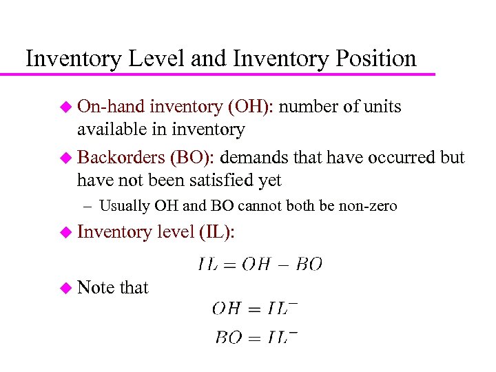6 Inventory Level and Inventory Position u On-hand inventory (OH): number of units available in inventory u Backorders (BO): demands that have occurred but have not been satisfied yet – Usually OH and BO cannot both be non-zero u Inventory u Note that level (IL):

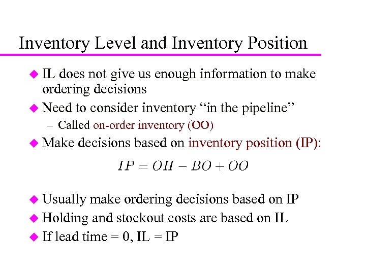7 Inventory Level and Inventory Position u IL does not give us enough information to make ordering decisions u Need to consider inventory “in the pipeline” – Called on-order inventory (OO) u Make decisions based on inventory position (IP): u Usually make ordering decisions based on IP u Holding and stockout costs are based on IL u If lead time = 0, IL = IP

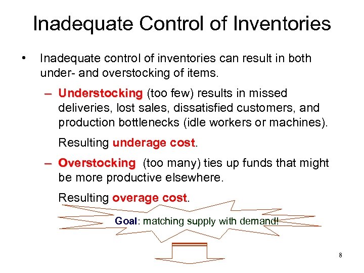Inadequate Control of Inventories • Inadequate control of inventories can result in both under- and overstocking of items. – Understocking (too few) results in missed deliveries, lost sales, dissatisfied customers, and production bottlenecks (idle workers or machines). Resulting underage cost. – Overstocking (too many) ties up funds that might be more productive elsewhere. Resulting overage cost. Goal: matching supply with demand! 8

Objective of Inventory Control Two fundamental decisions: ü When to order (timing) ü How much to order (size) 9

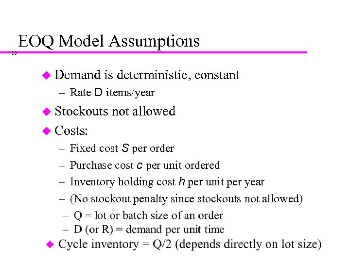10 EOQ Model Assumptions u Demand is deterministic, constant – Rate D items/year u Stockouts not allowed u Costs: – – Fixed cost S per order Purchase cost c per unit ordered Inventory holding cost h per unit per year (No stockout penalty since stockouts not allowed)

EOQ Model Inventory Level Optimal Order Quantity (Q*) Average Inventory (Q*/2) Reorder Point (ROP) Lead Time 11

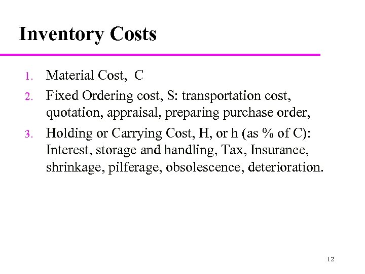Inventory Costs 1. 2. 3. Material Cost, C Fixed Ordering cost, S: transportation cost, quotation, appraisal, preparing purchase order, Holding or Carrying Cost, H, or h (as % of C): Interest, storage and handling, Tax, Insurance, shrinkage, pilferage, obsolescence, deterioration. 12

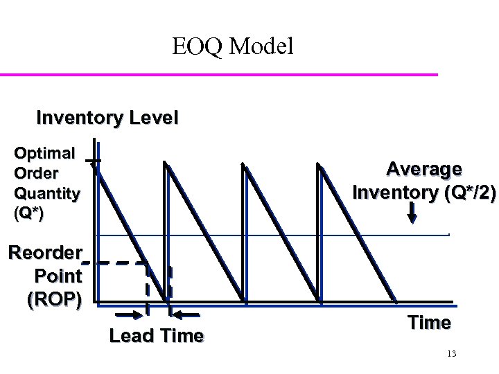EOQ Model Inventory Level Optimal Order Quantity (Q*) Average Inventory (Q*/2) Reorder Point (ROP) Lead Time 13

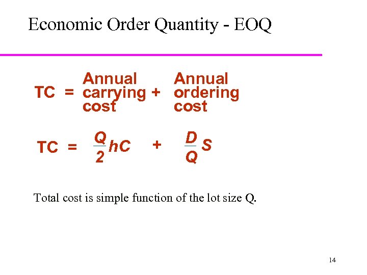Economic Order Quantity - EOQ Annual TC = carrying + ordering cost Q h. C TC = 2 + DS Q Total cost is simple function of the lot size Q. 14

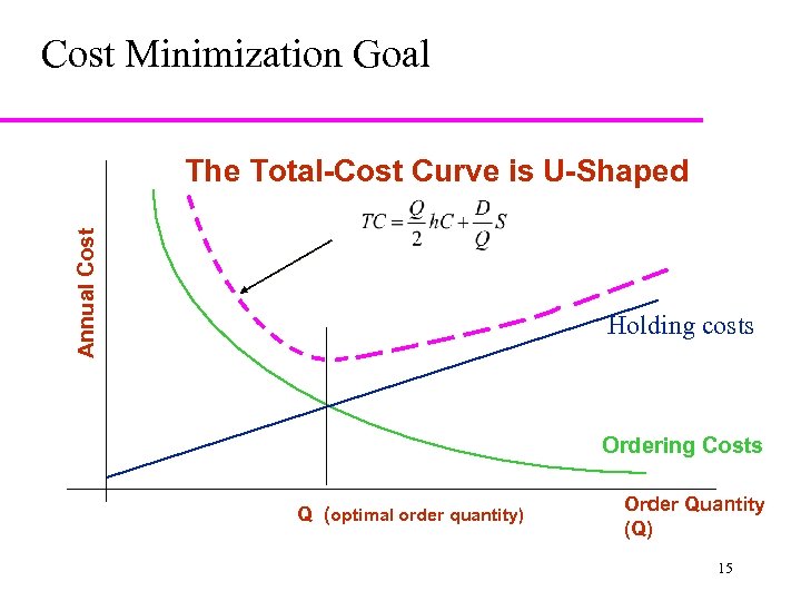Cost Minimization Goal Annual Cost The Total-Cost Curve is U-Shaped Holding costs Ordering Costs Q (optimal order quantity) Order Quantity (Q) 15

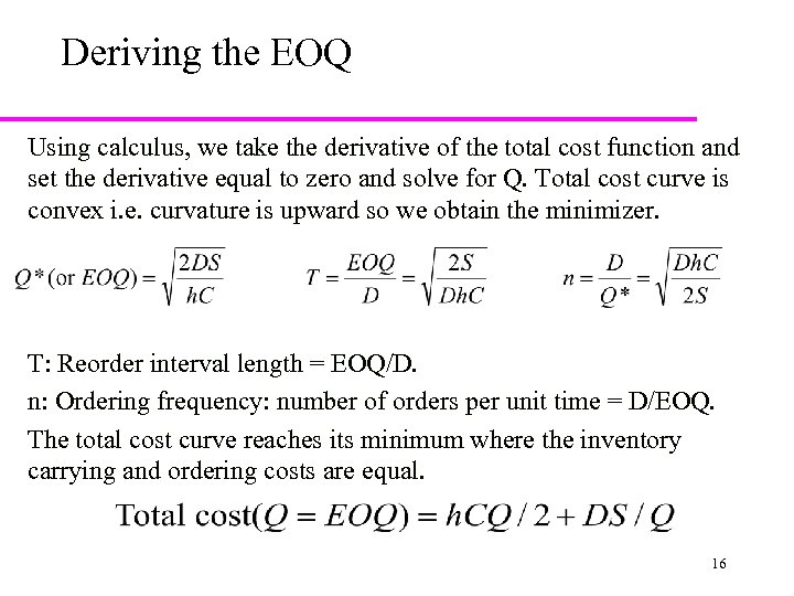Deriving the EOQ Using calculus, we take the derivative of the total cost function and set the derivative equal to zero and solve for Q. Total cost curve is convex i. e. curvature is upward so we obtain the minimizer. T: Reorder interval length = EOQ/D. n: Ordering frequency: number of orders per unit time = D/EOQ. The total cost curve reaches its minimum where the inventory carrying and ordering costs are equal. 16

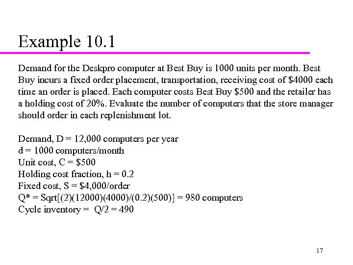Example 10. 1 Demand for the Deskpro computer at Best Buy is 1000 units per month. Best Buy incurs a fixed order placement, transportation, receiving cost of $4000 each time an order is placed. Each computer costs Best Buy $500 and the retailer has a holding cost of 20%. Evaluate the number of computers that the store manager should order in each replenishment lot. Demand, D = 12, 000 computers per year d = 1000 computers/month Unit cost, C = $500 Holding cost fraction, h = 0. 2 Fixed cost, S = $4, 000/order Q* = Sqrt[(2)(12000)(4000)/(0. 2)(500)] = 980 computers Cycle inventory = Q/2 = 490 17

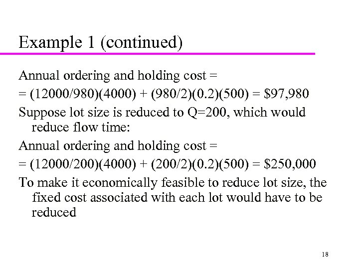Example 1 (continued) Annual ordering and holding cost = = (12000/980)(4000) + (980/2)(0. 2)(500) = $97, 980 Suppose lot size is reduced to Q=200, which would reduce flow time: Annual ordering and holding cost = = (12000/200)(4000) + (200/2)(0. 2)(500) = $250, 000 To make it economically feasible to reduce lot size, the fixed cost associated with each lot would have to be reduced 18

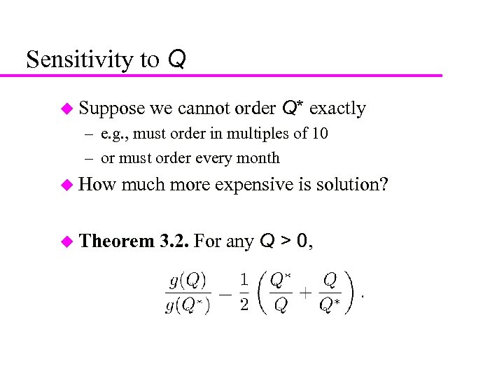19 Sensitivity to Q u Suppose we cannot order Q* exactly – e. g. , must order in multiples of 10 – or must order every month u How much more expensive is solution? u Theorem 3. 2. For any Q > 0,

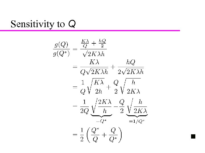20 Sensitivity to Q

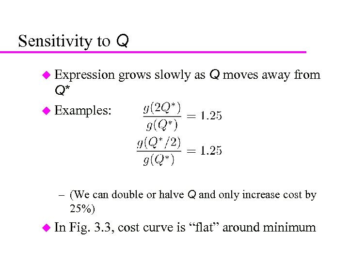21 Sensitivity to Q u Expression grows slowly as Q moves away from Q* u Examples: – (We can double or halve Q and only increase cost by 25%) u In Fig. 3. 3, cost curve is “flat” around minimum

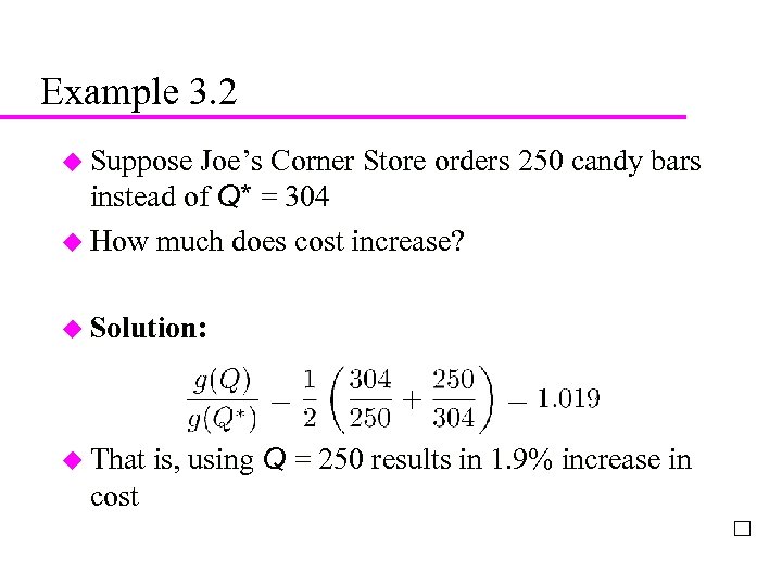22 Example 3. 2 u Suppose Joe’s Corner Store orders 250 candy bars instead of Q* = 304 u How much does cost increase? u Solution: u That cost is, using Q = 250 results in 1. 9% increase in

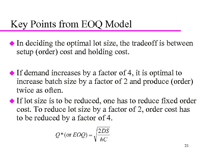Key Points from EOQ Model u In deciding the optimal lot size, the tradeoff is between setup (order) cost and holding cost. u If demand increases by a factor of 4, it is optimal to increase batch size by a factor of 2 and produce (order) twice as often. u If lot size is to be reduced, one has to reduce fixed order cost. To reduce lot size by a factor of 2, order cost has to be reduced by a factor of 4. 23

Aggregating Multiple Products in a Single Order u u Transportation is a significant contributor to the fixed cost per order Can possibly combine shipments of different products from the same supplier Can also have a single delivery coming from multiple suppliers or a single truck delivering to multiple retailers Aggregating across products, retailers, or suppliers in a single order allows for a reduction in lot size for individual products because fixed ordering and transportation costs are now spread across multiple products, retailers, or suppliers 24

Lot Sizing with Multiple Products or Customers u u In practice, the fixed ordering cost is dependent at least in part on the variety associated with an order of multiple models – A portion of the cost is related to transportation (independent of variety) – A portion of the cost is related to loading and receiving (not independent of variety) – Two scenarios: – Lots are ordered and delivered independently for each product – Lots are ordered and delivered jointly for all three models 25

Ex 3 Best Buy sells three models of computers, the Litepro, Medpro, and Heavypro. Annual demands for the three products are DL=12000 for the Litepro, DM=1200 for the Medpro, and DH=120 for the Heavypro. Assume that each model costs Best Buy $500. A fixed transportation cost of $4000 is incurred each time an order is delivered. For each model ordered and delivered on the same truck, an additional fixed cost of $1000 is incurred for receiving and storage. Best Buy incurs a holding cost of 20%. Evaluate the lot sizes that the Best Buy manager should order if lots for each product are ordered and delivered independently. Also evaluate the annual cost of such a policy. 26

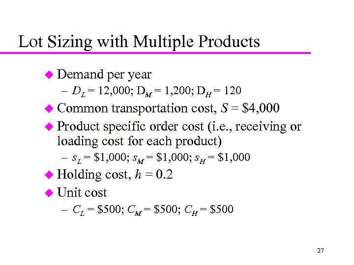Lot Sizing with Multiple Products u Demand per year – DL = 12, 000; DM = 1, 200; DH = 120 u Common transportation cost, S = $4, 000 u Product specific order cost (i. e. , receiving or loading cost for each product) – s. L = $1, 000; s. M = $1, 000; s. H = $1, 000 u Holding cost, h = 0. 2 u Unit cost – CL = $500; CM = $500; CH = $500 27

Delivery Options u No Aggregation: Each product ordered separately u Complete Aggregation: All products delivered on each truck 28

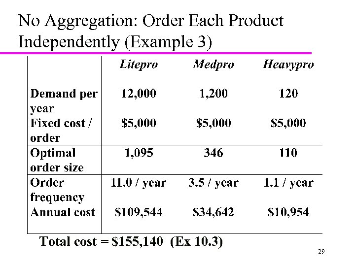No Aggregation: Order Each Product Independently (Example 3) Total cost = $155, 140 (Ex 10. 3) 29

Ex 10. 4 Consider the Best Buy data in Example 3. The three product managers have decided to aggregate and order all three models each time they place an order. Evaluate the optimal lot size for each model. 30

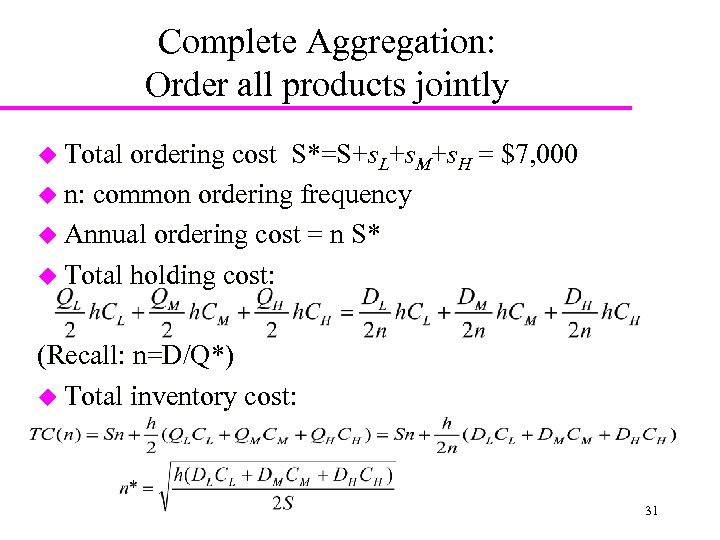Complete Aggregation: Order all products jointly u Total ordering cost S*=S+s. L+s. M+s. H = $7, 000 u n: common ordering frequency u Annual ordering cost = n S* u Total holding cost: (Recall: n=D/Q*) u Total inventory cost: 31

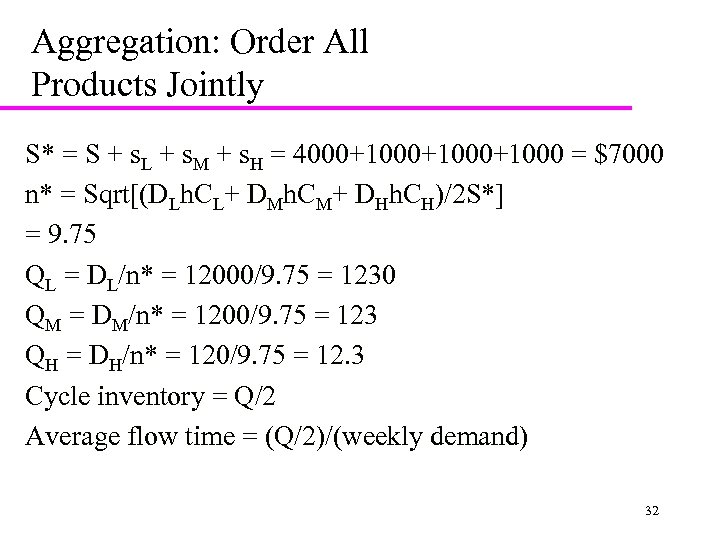Aggregation: Order All Products Jointly S* = S + s. L + s. M + s. H = 4000+1000+1000 = $7000 n* = Sqrt[(DLh. CL+ DMh. CM+ DHh. CH)/2 S*] = 9. 75 QL = DL/n* = 12000/9. 75 = 1230 QM = DM/n* = 1200/9. 75 = 123 QH = DH/n* = 120/9. 75 = 12. 3 Cycle inventory = Q/2 Average flow time = (Q/2)/(weekly demand) 32

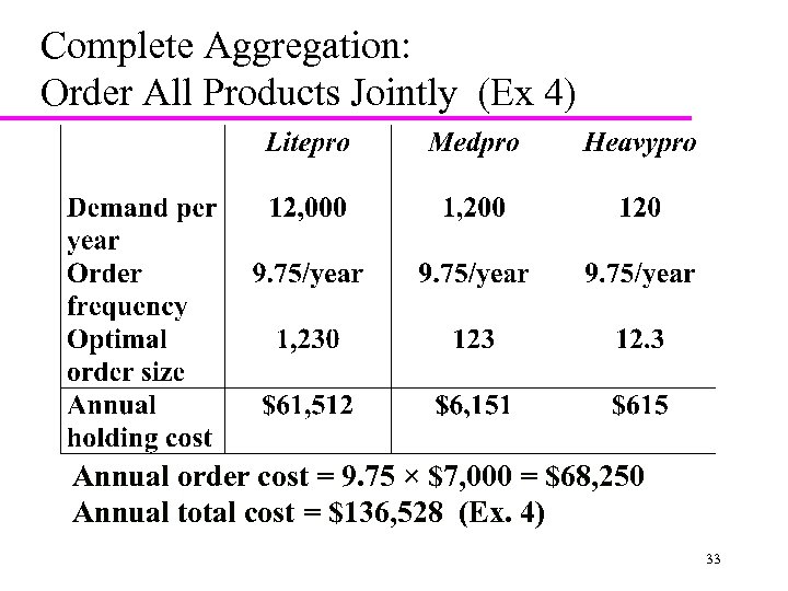Complete Aggregation: Order All Products Jointly (Ex 4) Annual order cost = 9. 75 × $7, 000 = $68, 250 Annual total cost = $136, 528 (Ex. 4) 33

Lessons from Aggregation u Aggregation allows firm to lower lot size without increasing cost u Complete aggregation is effective if product specific fixed cost is a small fraction of joint fixed cost 34

Power-of-Two Policies 35 u Suppose we are given a base period – Week, day, work shift, etc. interval T must be power-of-two multiple of base period u Order – Place orders every 1 day, or 2 days, or 4 days, or… – Or every ½ day, or every ¼ day, or… u Key questions: – What order interval should we use? – How much more expensive than optimal T ? © 2014 Lawrence V. Snyder

Why Power-of-Two? 36 u Simpler ordering schedule u Easier coordination in multi-stage systems – – e. g. , one-warehouse, multi-retailer (OWMR) problem Retailers’ orders to central warehouse line up Optimal policy for OWMR is not known Power-of-two policies known to be close to optimal (Roundy 1985, Muckstadt and Roundy 1993) – More on this later in course u Mathematical © 2014 Lawrence V. Snyder convenience

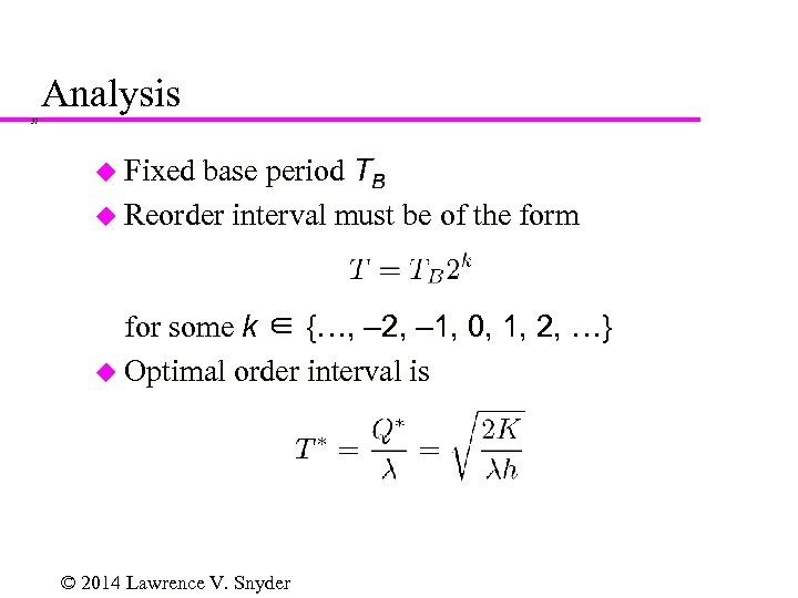Analysis 37 base period TB u Reorder interval must be of the form u Fixed for some k ∈ {…, – 2, – 1, 0, 1, 2, …} u Optimal order interval is © 2014 Lawrence V. Snyder

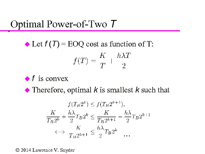Optimal Power-of-Two T 38 u Let f (T) = EOQ cost as function of T: uf is convex u Therefore, optimal k is smallest k such that … © 2014 Lawrence V. Snyder

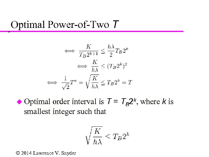Optimal Power-of-Two T 39 order interval is T = TB 2 k, where k is smallest integer such that u Optimal © 2014 Lawrence V. Snyder

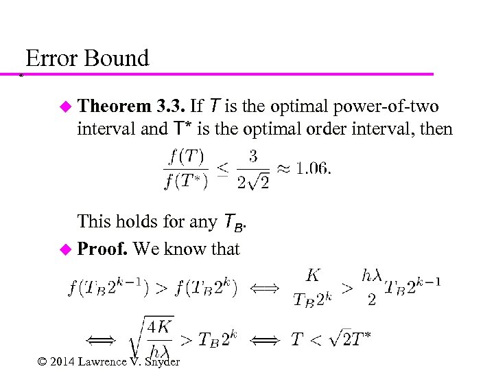Error Bound 40 3. 3. If T is the optimal power-of-two interval and T* is the optimal order interval, then u Theorem This holds for any TB. u Proof. We know that © 2014 Lawrence V. Snyder

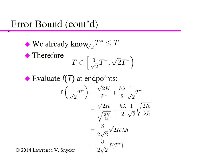Error Bound (cont’d) 41 u We already know u Therefore u Evaluate f(T) at endpoints: © 2014 Lawrence V. Snyder

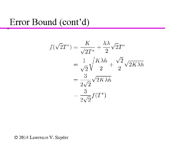Error Bound (cont’d) 42 © 2014 Lawrence V. Snyder

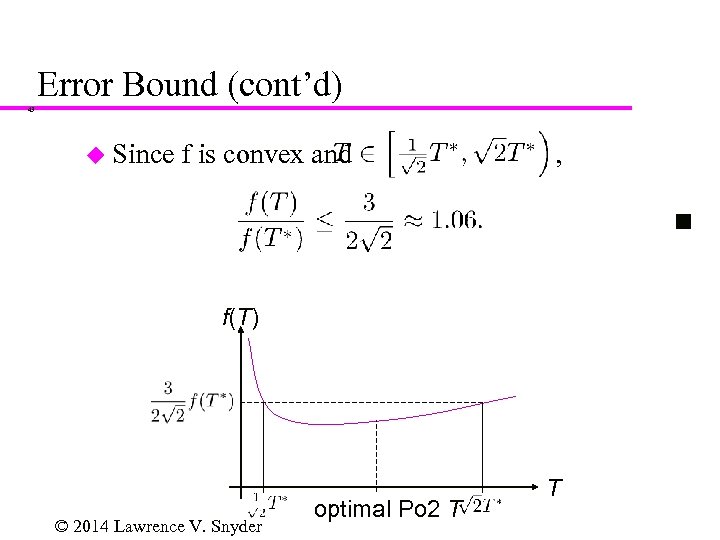Error Bound (cont’d) 43 u Since f is convex and , f(T) © 2014 Lawrence V. Snyder optimal Po 2 T T

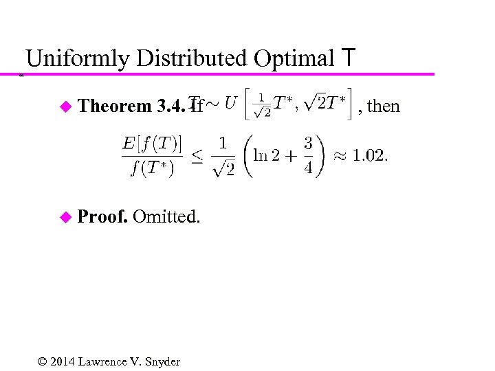Uniformly Distributed Optimal T 44 u Theorem u Proof. 3. 4. If Omitted. © 2014 Lawrence V. Snyder , then

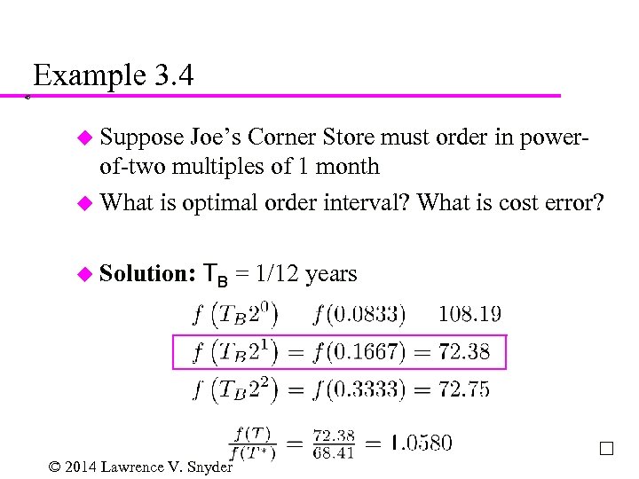Example 3. 4 45 u Suppose Joe’s Corner Store must order in powerof-two multiples of 1 month u What is optimal order interval? What is cost error? u Solution: TB = 1/12 years © 2014 Lawrence V. Snyder

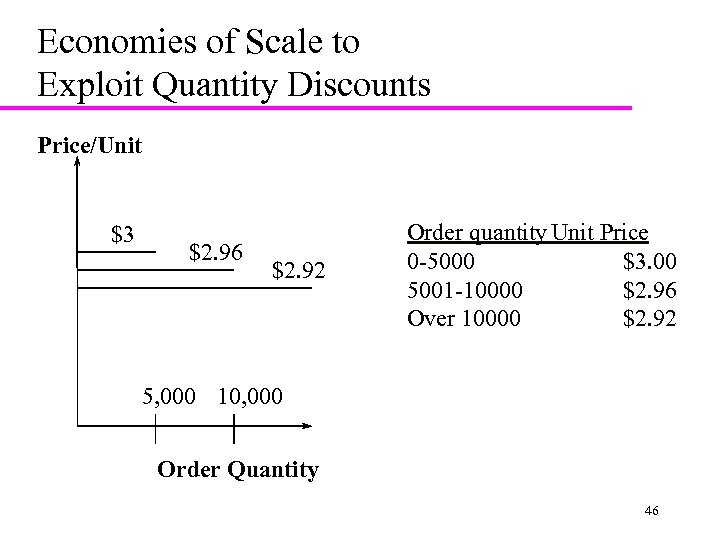Economies of Scale to Exploit Quantity Discounts Price/Unit $3 $2. 96 $2. 92 Order quantity Unit Price 0 -5000 $3. 00 5001 -10000 $2. 96 Over 10000 $2. 92 5, 000 10, 000 Order Quantity 46

Economies of Scale to Exploit Quantity Discounts u Given a price schedule with quantity discounts, what is the optimal purchasing decision for a buyer seeking to maximize profits ? 47

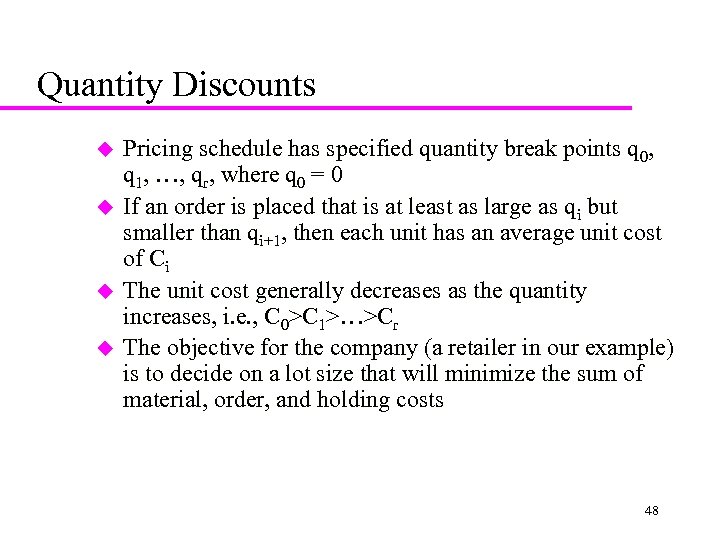Quantity Discounts u u Pricing schedule has specified quantity break points q 0, q 1, …, qr, where q 0 = 0 If an order is placed that is at least as large as qi but smaller than qi+1, then each unit has an average unit cost of Ci The unit cost generally decreases as the quantity increases, i. e. , C 0>C 1>…>Cr The objective for the company (a retailer in our example) is to decide on a lot size that will minimize the sum of material, order, and holding costs 48

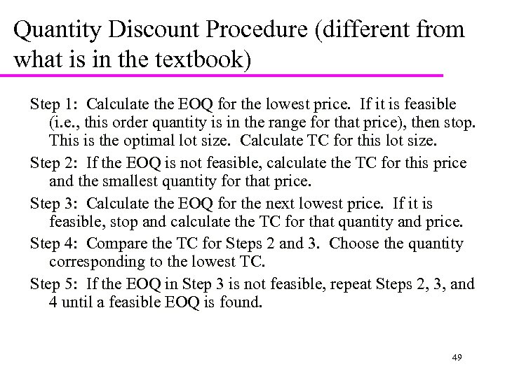Quantity Discount Procedure (different from what is in the textbook) Step 1: Calculate the EOQ for the lowest price. If it is feasible (i. e. , this order quantity is in the range for that price), then stop. This is the optimal lot size. Calculate TC for this lot size. Step 2: If the EOQ is not feasible, calculate the TC for this price and the smallest quantity for that price. Step 3: Calculate the EOQ for the next lowest price. If it is feasible, stop and calculate the TC for that quantity and price. Step 4: Compare the TC for Steps 2 and 3. Choose the quantity corresponding to the lowest TC. Step 5: If the EOQ in Step 3 is not feasible, repeat Steps 2, 3, and 4 until a feasible EOQ is found. 49

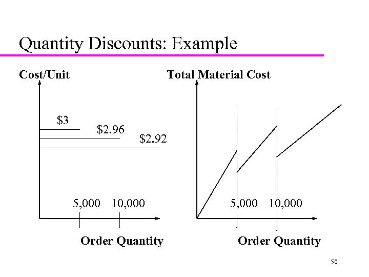Quantity Discounts: Example Cost/Unit $3 Total Material Cost $2. 96 $2. 92 5, 000 10, 000 Order Quantity 50

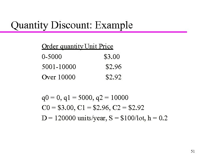Quantity Discount: Example Order quantity Unit Price 0 -5000 $3. 00 5001 -10000 $2. 96 Over 10000 $2. 92 q 0 = 0, q 1 = 5000, q 2 = 10000 C 0 = $3. 00, C 1 = $2. 96, C 2 = $2. 92 D = 120000 units/year, S = $100/lot, h = 0. 2 51

All-Unit Quantity Discount: Example Step 1: Calculate Q 2* = Sqrt[(2 DS)/h. C 2] = Sqrt[(2)(120000)(100)/(0. 2)(2. 92)] = 6410 Not feasible (6410 < 10001) Calculate TC 2 using C 2 = $2. 92 and q 2 = 10001 TC 2 = (120000/10001)(100)+(10001/2)(0. 2)(2. 92)+(120000)(2. 92) = $354, 520 Step 2: Calculate Q 1* = Sqrt[(2 DS)/h. C 1] =Sqrt[(2)(120000)(100)/(0. 2)(2. 96)] = 6367 Feasible (5000<6367<10000) Stop TC 1 = (120000/6367)(100)+(6367/2)(0. 2)(2. 96)+(120000)(2. 96) = $358, 969 TC 2 < TC 1 The optimal order quantity Q* is q 2 = 10001 52

Why Quantity Discounts? u Coordination in the supply chain 10 -53

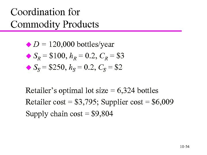Coordination for Commodity Products u. D = 120, 000 bottles/year u SR = $100, h. R = 0. 2, CR = $3 u SS = $250, h. S = 0. 2, CS = $2 Retailer’s optimal lot size = 6, 324 bottles Retailer cost = $3, 795; Supplier cost = $6, 009 Supply chain cost = $9, 804 10 -54

Coordination for Commodity Products u What can the supplier do to decrease supply chain costs? – Coordinated lot size: 9, 165; Retailer cost = $4, 059; Supplier cost = $5, 106; Supply chain cost = $9, 165 u Effective pricing schemes – quantity discount 10 -55

Quantity Discounts When Firm Has Market Power The annual demand faced by a retailer is given by the demand curve 360, 000 -60, 000 p, where p is the price at which the retailer sells a type of product. The manufacturer incurs a production cost of c=$2 per product. The manufacturer must decide on price (w) to charge the retailer, and the retailer in turn must decide on the price (p) to charge the customer. What are the optimal w for the manufacturer to charge the retailer and the optimal retail price p for the retailer to charge customer? 10 -56

Quantity Discounts When Firm Has Market Power u No inventory related costs u Demand curve 360, 000 - 60, 000 p What are the optimal prices and profits in the following situations? – The two stages make the pricing decision independently » Price = $5, Profit = $180, 000, Demand = 60, 000 – The two stages coordinate the pricing decision » Price = $4, Profit = $240, 000, Demand = 120, 000 10 -57

Design a volume discount scheme that achieves the coordinated solution u Design a volume discount scheme that achieves the coordinated solution 10 -58

Production Order Quantity Model 59

60

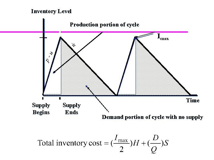Inventory Level Production portion of cycle Imax p- u -u Supply Begins Supply Ends Time Demand portion of cycle with no supply

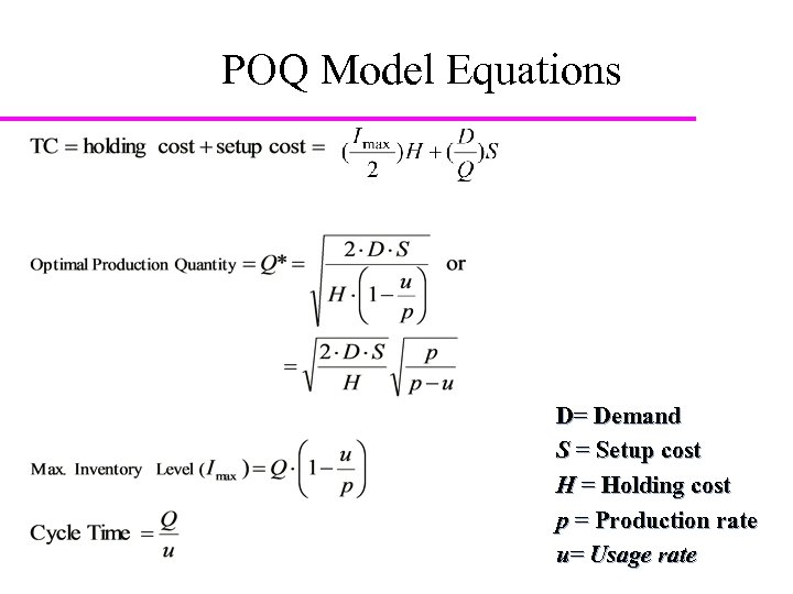
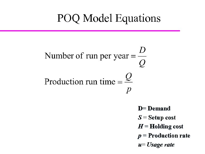
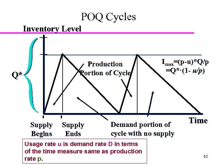POQ Cycles Inventory Level Production Portion of Cycle Q* Supply Begins Supply Ends Imax=(p-u)*Q/p =Q*·(1 - u/p) Demand portion of cycle with no supply Usage rate u is demand rate D in terms of the time measure same as production rate p. Time 62

POQ Model Equations D= Demand S = Setup cost H = Holding cost p = Production rate u= Usage rate

POQ Model Equations D= Demand S = Setup cost H = Holding cost p = Production rate u= Usage rate

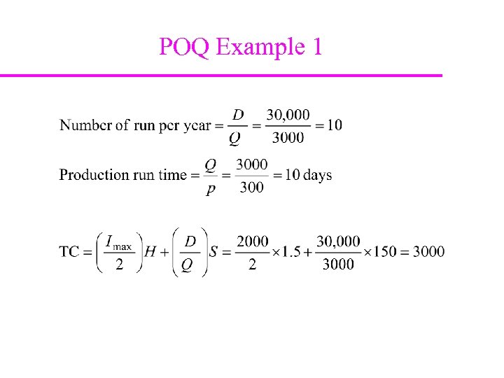
POQ Example 1 You’re a production planner for Stanley Tools faces an annual demand of 30, 000 units of screw. The production rate is 300 units per day with 300 working days a year. Production setup cost is $150 per order. Carrying cost is $1. 50 per screw driver. What is the optimal lot size? D= Demand = 30, 000/yr S= Setup cost = $150 H = Holding cost = $1. 5/unit/yr p = Production per day = 300/day u=usage rate per day=30, 000/300=100/day

POQ Example 1 Optimal lot size:

POQ Example 1

68 3. 3 Periodic Review: The Wagner. Whitin Model © 2014 Lawrence V. Snyder

Problem Statement 69 The Wagner-Whitin Model Wagner and Whitin (1958) Similarities to EOQ Fixed order cost Stockouts not allowed Choose order quantity to minimize total cost Differences from EOQ Periodic review Demand may change over time © 2014 Lawrence V. Snyder

Problem Statement (cont’d) 70 T-period, finite-horizon model Lead time = 0 May not be optimal to order in every period ZIO is optimal (we will show) Therefore, need to choose how many whole periods’ of demand to order each time we order In each period, decide whether to order And if so, how much © 2014 Lawrence V. Snyder

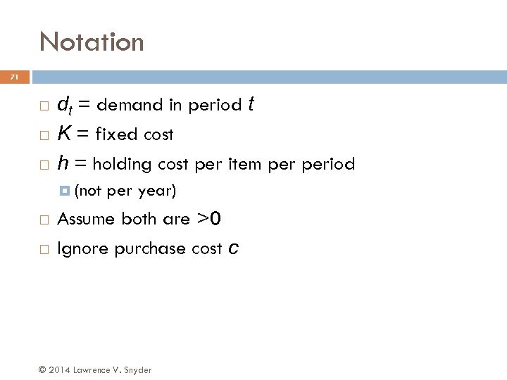Notation 71 dt = demand in period t K = fixed cost h = holding cost per item period (not per year) Assume both are >0 Ignore purchase cost c © 2014 Lawrence V. Snyder

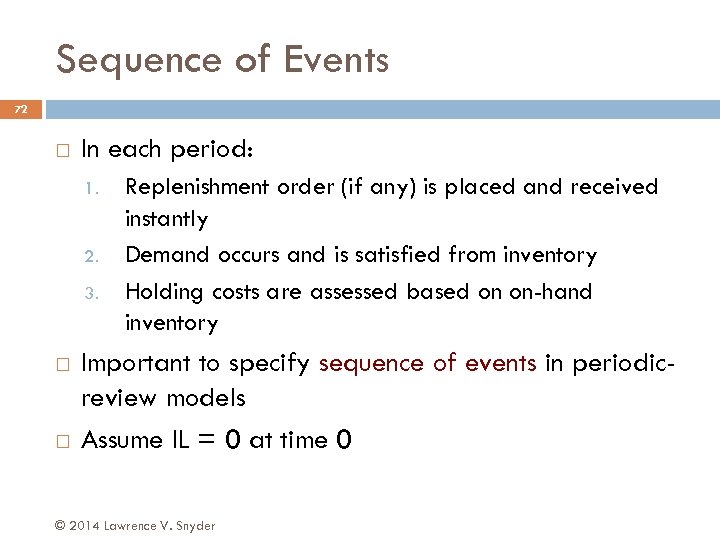Sequence of Events 72 In each period: 1. 2. 3. Replenishment order (if any) is placed and received instantly Demand occurs and is satisfied from inventory Holding costs are assessed based on on-hand inventory Important to specify sequence of events in periodicreview models Assume IL = 0 at time 0 © 2014 Lawrence V. Snyder

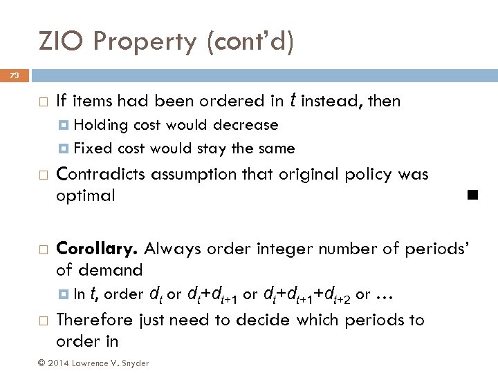ZIO Property (cont’d) 73 If items had been ordered in t instead, then Holding cost would decrease Fixed cost would stay the same Contradicts assumption that original policy was optimal Corollary. Always order integer number of periods’ of demand In t, order dt or dt+dt+1+dt+2 or … Therefore just need to decide which periods to order in © 2014 Lawrence V. Snyder

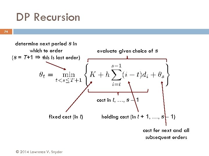DP Recursion 74 determine next period s in which to order (s = T+1 ⇒ this is last order) evaluate given choice of s cost in t, …, s – 1 fixed cost (in t) holding cost (in t + 1, …, s – 1) cost for next and all subsequent orders © 2014 Lawrence V. Snyder

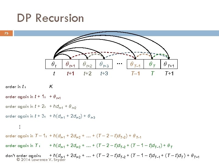DP Recursion 75 θt θ t+2 θ t+3 t order in t : θ t+1 t+2 t+3 … θ T– 1 θT θ T+1 T– 1 T T+1 K order again in t + 1: + θ t+1 order again in t + 2: + hdt+1 + θ t+2 order again in t + 3: + h(dt+1 + 2 dt+2) + θ t+3 … order again in T – 1: + h(dt+1 + 2 dt+2 + … + (T – 2 – t)d. T– 2) + θ T– 1 order again in T : + h(dt+1 + 2 dt+2 + … + (T – 2 – t)d. T– 2 + (T – 1 – t)d. T– 1) + θ T don’t order again: + h(dt+1 + 2 dt+2 + … + (T – 2 – t)d. T– 2 + (T – 1 – t)d. T– 1 + (T – t)d. T ) + θ T+1 © 2014 Lawrence V. Snyder

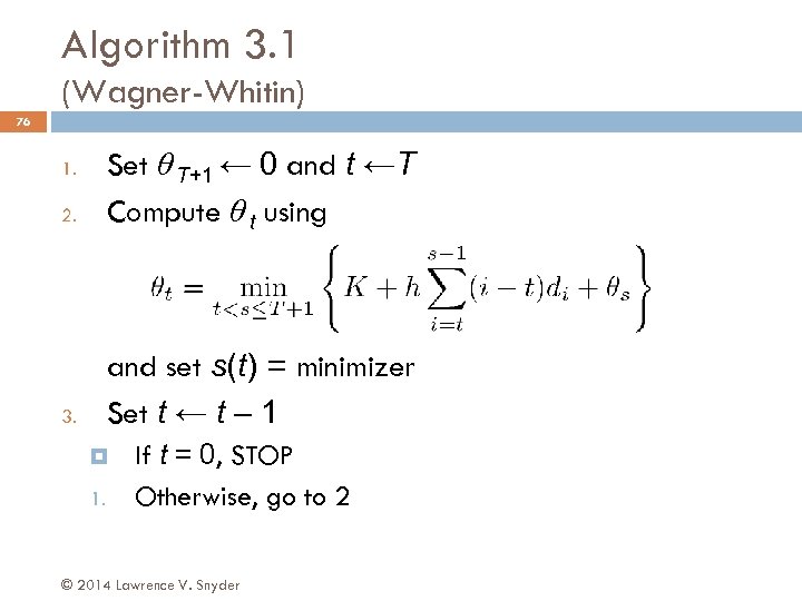Algorithm 3. 1 (Wagner-Whitin) 76 2. Set θ T+1 ← 0 and t ←T Compute θ t using 3. and set s(t) = minimizer Set t ← t – 1 1. 1. If t = 0, STOP Otherwise, go to 2 © 2014 Lawrence V. Snyder

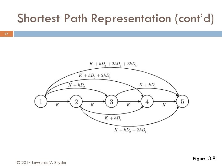Shortest Path Representation (cont’d) 77 © 2014 Lawrence V. Snyder Figure 3. 9

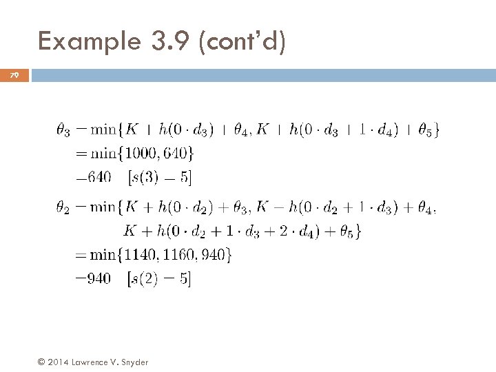
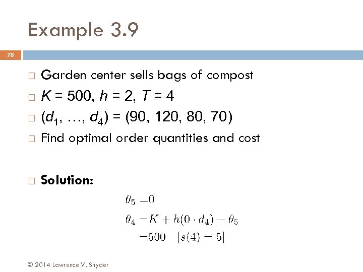Example 3. 9 78 Garden center sells bags of compost K = 500, h = 2, T = 4 (d 1, …, d 4) = (90, 120, 80, 70) Find optimal order quantities and cost Solution: © 2014 Lawrence V. Snyder

Example 3. 9 (cont’d) 79 © 2014 Lawrence V. Snyder

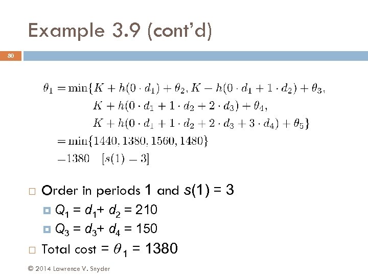Example 3. 9 (cont’d) 80 Order in periods 1 and s(1) = 3 Q 1 = d 1+ d 2 = 210 Q 3 = d 3+ d 4 = 150 Total cost = θ 1 = 1380 © 2014 Lawrence V. Snyder