

04c434b076c02327e1a71825e39a7619.ppt
- Количество слайдов: 76
 Chapter 3 Demand for Health Care Services
 Outline Introduction of health insurance p Theoretical model of health insurance p Empirical estimates of demand from the literature p Practice problems p The RAND Health Insurance Experiment p Example: Interpreting results from a regression on abortion demand p
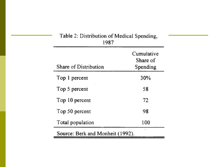
 Why Health Insurance? p Medical expenditure is extreme volatile n n n 1% use 25% exp 5% use 50% exp 20% use 75% exp p Difficult to self-insured because some people are sicker than others p Health insurance is relatively new (at the end of 19 th century) since treatment was not very effective before
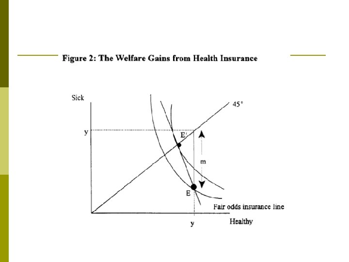
 Formalizing This Intuition: Expected Utility Model p Let p stand for the probability of an adverse event. Then expected utility is: p Where C 0 and C 1 stand for consumption in the good and bad states of the world, respectively.
 Formalizing This Intuition: Expected Utility Model p p This model can be used to examine the individual’s demand for insurance. Imagine, for example, that there was a 1% chance that Sam will get into an accident that caused $30, 000 in damages. n n n Sam can insure some, none, or all of these medical expenses. The policy costs m¢ per $1 of coverage. If Sam buys a policy that pays him $b in an accident, his premium is $mb. Full insurance in this case would cost m x $30, 000. p In the state of the world where Sam does get hit, he will be $b-$mb richer than if he hadn’t bought insurance. p If he doesn’t get hit by the car, he will be $mb poorer than he otherwise would have been.
 Formalizing This Intuition: Expected Utility Model That is, the insurance policy translates Sam’s consumption from periods when it is high to periods when it is low. p Sam’s desire to buy the policy depends on the price that is charged. p An actuarially fair premium the price charged equal sets to the expected payout. p
 Formalizing This Intuition: Expected Utility Model In this case, the expected payout is $30, 000 x 1%, or $300 per policy. So a $300 premium is actuarially fair. p With actuarially fair pricing, individuals will want to fully insure themselves to equalize consumption in all states of the world. p
 Formalizing This Intuition: Expected Utility Model p Consider the case, for example, when the utility function is: p Also assume that C 0=30, 000. Then expected utility without insurance is:
 Formalizing This Intuition: Expected Utility Model p If, instead, you bought actuarially fair insurance for $300, expected utility is: p Utility is higher, even though the odds are that the premium was paid for nothing. This is because you would rather have equal consumption regardless of the accident, rather than a very low level in the bad state of the world. This is illustrated in Table 1. 1
 Table 1 The expected utility model And Sam is … Consu mption Utility √C Not hit by a car (D=99%) $30, 000 173. 2 Hit by a car (D=1%) 0 0 Buys full insurance (for $300) Not hit by a car (D=99%) $29, 700 172. 3 Hit by a car (D=1%) $29, 700 172. 3 Buys partial insurance (for $150) Not hit by a car (D=99%) $29, 850 172. 8 Hit by a car (D=1%) $14, 850 121. 8 If Sam … Doesn’t buy insurance Expected utility 0. 99 x 173. 2 + 0. 01 x 0 = 171. 5 0. 99 x 172. 3 + 0. 01 x 172. 3 = 172. 3 0. 99 x 172. 8 + 0. 01 x 121. 8 = 172. 2
 Formalizing This Intuition: Expected Utility Model The central result of expected utility theory is that with actuarially fair pricing, individuals will want to fully insure themselves to equalize consumption in all states of the world. p Clearly Sam’s utility is higher in row 2, with full insurance, than in row 1, with no insurance. p Yet, Sam also prefers full insurance to any other level of benefits. Row 3, which shows coverage for half of the costs of the accident, gives lower expected utility. p
 Formalizing This Intuition: Expected Utility Model Thus, even if insurance is expensive, so long as the price (premium) is actuarially fair, individuals will want to fully insure themselves against adverse events. p The implication: the efficient market outcome is full insurance and thus full consumption smoothing. p
 The role of risk aversion p Risk aversion is the extent to which an individual is willing to bear risk. n n Risk averse individuals have a rapidly diminishing marginal utility of consumption; they are very afraid of consumption falling. Individuals with any degree of risk aversion will buy insurance when it is priced actuarially fairly. But when the insurance is not fair, some will choose to not buy insurance.
 Insurance with Fixed Spending p One person: n n p One illness n n n p U(x, h) U’>0, U’’<0 sick with probability p fixed treatment cost: m H(h, m)=H(1, m)=H(0, 0) Two states n n Sick (s): U(y-m, H(1, m)) Health (m): U(y, H(0, 0))
 Without insurance
 With insurance p Fair insurance: π= pm
 Comparing With and Without Insurance p Taking Taylor’s expansion, we have
 p The insurance plan specifies the amount of money transferred to the bad state
 Problem with Fixed Spending p Complete information n All the sicknesses known All the treatment known No wasted resources in the policy p The insurance specifies the amount of money being transferred during the sickness (contingency plan) p The policy completely insures the health, but s it possible to insure someone’s health?
 n n") Estimating Demand for Medical Care p Quantity demanded = f( … ) n n n n out-of-pocket price real income time costs prices of substitutes and complements tastes and preferences profile state of health quality of care
Estimating Demand for Medical Care p Quantity demanded = f( … ) n n n n out-of-pocket price real income time costs prices of substitutes and complements tastes and preferences profile state of health quality of care
 Empirical Evidence p Demand for primary care services (prevention, early detection, & treatment of disease) has been found to be price inelastic n n n Estimates tend to be in the -. 1 to -. 7 range A 10% in the out-of-pocket price of hospital or physician services leads to a 1 to 7% decrease in quantity demanded Ceteris paribus, total expenditures on hospital and physician services increase with a greater out-of-pocket price
 p Demand for other types of medical care is slightly") Empirical Evidence (cont. ) p Demand for other types of medical care is slightly more price elastic than demand for primary care p Consumers should be more price sensitive as the portion of the bill paid out of pocket increases
Empirical Evidence (cont. ) p Demand for other types of medical care is slightly more price elastic than demand for primary care p Consumers should be more price sensitive as the portion of the bill paid out of pocket increases
 Out-of-Pocket Payments in the U. S. l Hypothesis: Consumers are more price sensitive if they pay a larger % of the health care bill The fall in the % of out-of-pocket payments may explain the rapid rise in health care costs
 Out-of-Pocket Payments in the U. S. p l Total Expenditures and % Paid Out-of-Pocket, 2007 Hypothesis: Consumers are more price sensitive if they pay a larger % of the health care bill Higher hospital and physician expenditures may be due to the low % paid out-of-pocket
 p The previous 2 slides argue") Out-of-Pocket Payments in the U. S. (cont. ) p The previous 2 slides argue that: insurance coverage expenditures p But it may be the opposite: expenditures insurance coverage. p We cannot identify a causal effect using just this data
Out-of-Pocket Payments in the U. S. (cont. ) p The previous 2 slides argue that: insurance coverage expenditures p But it may be the opposite: expenditures insurance coverage. p We cannot identify a causal effect using just this data
 p Studies which have examined price and quantity variation within") Empirical Evidence (cont. ) p Studies which have examined price and quantity variation within service types have found that: n n The price elasticity of demand for dental services for females is -. 5 to -. 7 The own-price elasticity of demand for nursing home services is between -. 73 and -2. 4
Empirical Evidence (cont. ) p Studies which have examined price and quantity variation within service types have found that: n n The price elasticity of demand for dental services for females is -. 5 to -. 7 The own-price elasticity of demand for nursing home services is between -. 73 and -2. 4
 p At the individual level, the income elasticity of demand") Empirical Evidence (cont. ) p At the individual level, the income elasticity of demand for medical services is below +1. 0 p The travel time elasticity of demand is almost as large as the own-price elasticity of demand p Little consensus on whether hospital care and ambulatory physician services are substitutes or complements
Empirical Evidence (cont. ) p At the individual level, the income elasticity of demand for medical services is below +1. 0 p The travel time elasticity of demand is almost as large as the own-price elasticity of demand p Little consensus on whether hospital care and ambulatory physician services are substitutes or complements
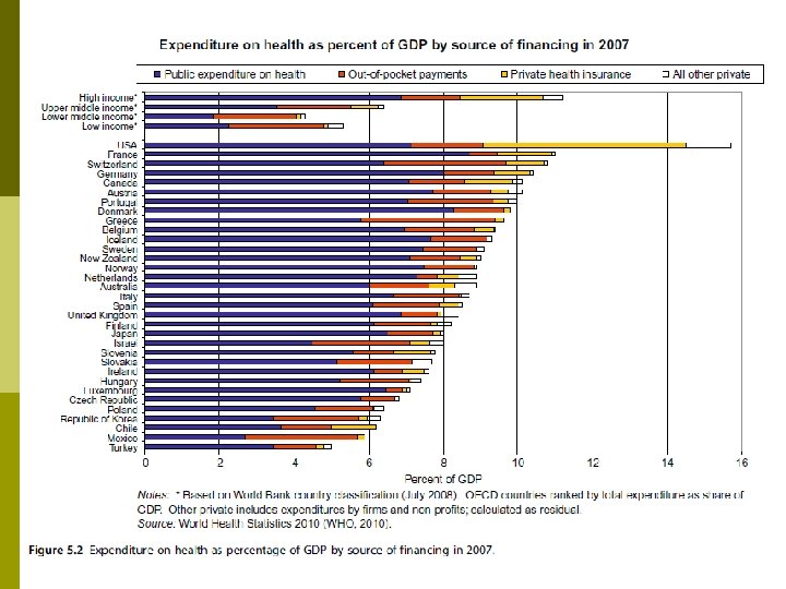
 International Estimates of Income Elasticity Are health care expenditures destined to consume a larger portion of GDP as GDP grows? p Regression Analysis p n Sample - developed countries Ln(Real per capita health expenditures) n = a+b Ln(Real per capita income) Estimates of b range between 1. 13 and 1. 31 +e
 Applying Demand Theory to Real Data Demand analyses in health care must take insurance into account p Demand analyses are critical in shaping managerial and public policy decisions p
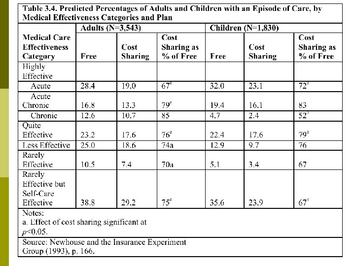
 p Research issues: n n p How does") The Rand Health Insurance Experiment (HIE) p Research issues: n n p How does cost sharing affect demand for personal health care services? How does cost sharing affect demand for particular services, e. g. , hospital care, dental services? Does use of personal health care services improve health? How does a change from fee-for-service payment to capitation affect demand for personal health care services? Rationale for studying HIE 30+ years after HIE completed
The Rand Health Insurance Experiment (HIE) p Research issues: n n p How does cost sharing affect demand for personal health care services? How does cost sharing affect demand for particular services, e. g. , hospital care, dental services? Does use of personal health care services improve health? How does a change from fee-for-service payment to capitation affect demand for personal health care services? Rationale for studying HIE 30+ years after HIE completed
 The Rand Health Insurance Experiment A large, social science experiment to study individuals’ medical care under insurance p A large sample of families were provided differing levels of health insurance coverage p n Researchers then studied their subsequent health care use
 The Sample p 5, 809 individuals, under 65 p 6 sites n Dayton OH, Seattle WA, Fitchburg MA, n Charlston SC, Georgetown County SC, Franklin County MA p 1974 – 1977 p Cost : $80 million
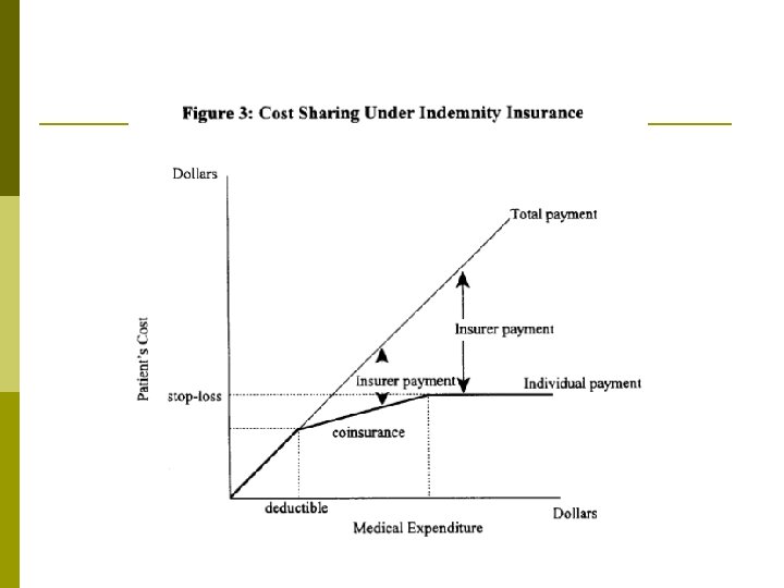
 Insurance Plans in the Experiment p Families randomly assigned to 1 of 14 insurance plans differing in cost sharing rates and in maximum dollar expenditures per year (MDE or stop loss) Free fee-for-service (FFS). - i. e. , no coinsurance p 25% copayment per physician visit p 50% copayment per physician visit p 95% copayment per physician visit p
 Insurance Plans in the Experiment p Individual deductible - $150 deductible for physician visits; all subsequent visits free p HMO - Not the same as free fee-for-service - Since HMO receives a fixed annual fee, it seeks to limit physician visits
 Table 3. 3. Sample Means for Annual Use of Medical Services per Capita Plans* Free 25% 50% 95% individual deductible Outpatient Face-to. Expenses Face Visits (1984 $) 4. 55 340 3. 33 260 3. 03 224 2. 73 203 3. 02 235 Inpatient Dollars (1984 $) 409 373 450 315 373 Total Probability Expenses Using Any (1984 $) Medical Service 749 86. 8 634 78. 8 674 77. 2 518 67. 7 608 72. 3 * The chi-square test was used to test the null hypothesis of no difference among the five plan means. In each instance, the chi-square statistic was significant to at least 5 percent level. The only exception was for inpatient dollars Source : Willard G. Manning et al. “Health Insurance and the Demand for Medical Care : Evidence from a Randomized Experiment, ” American Economic Review 77 (June 1987), Table 2
 Table 3. 3. Sample Means for Annual Use of Medical Services per Capita Plans* Free 25% 50% 95% individual deductible Outpatient Face-to. Expenses Face Visits (1984 $) 4. 55 340 3. 33 260 3. 03 224 2. 73 203 3. 02 235 Inpatient Dollars (1984 $) 409 373 450 315 373 Total Probability Expenses Using Any (1984 $) Medical Service 749 86. 8 634 78. 8 674 77. 2 518 67. 7 608 72. 3 * The chi-square test was used to test the null hypothesis of no difference among the five plan means. In each instance, the chi-square statistic was significant to at least 5 percent level. The only exception was for inpatient dollars Source : Willard G. Manning et al. “Health Insurance and the Demand for Medical Care : Evidence from a Randomized Experiment, ” American Economic Review 77 (June 1987), Table 2
 Table 3. 3. Sample Means for Annual Use of Medical Services per Capita Plans* Free 25% 50% 95% individual deductible Outpatient Face-to. Expenses Face Visits (1984 $) 4. 55 340 3. 33 260 3. 03 224 2. 73 203 3. 02 235 Inpatient Dollars (1984 $) 409 373 450 315 373 Total Probability Expenses Using Any (1984 $) Medical Service 749 86. 8 634 78. 8 674 77. 2 518 67. 7 608 72. 3 * The chi-square test was used to test the null hypothesis of no difference among the five plan means. In each instance, the chi-square statistic was significant to at least 5 percent level. The only exception was for inpatient dollars Source : Willard G. Manning et al. “Health Insurance and the Demand for Medical Care : Evidence from a Randomized Experiment, ” American Economic Review 77 (June 1987), Table 2
 Table 3. 3. Sample Means for Annual Use of Medical Services per Capita Plans* Free 25% 50% 95% individual deductible Outpatient Face-to. Expenses Face Visits (1984 $) 4. 55 340 3. 33 260 3. 03 224 2. 73 203 3. 02 235 Inpatient Dollars (1984 $) 409 373 450 315 373 Total Probability Expenses Using Any (1984 $) Medical Service 749 86. 8 634 78. 8 674 77. 2 518 67. 7 608 72. 3 * The chi-square test was used to test the null hypothesis of no difference among the five plan means. In each instance, the chi-square statistic was significant to at least 5 percent level. The only exception was for inpatient dollars Source : Willard G. Manning et al. “Health Insurance and the Demand for Medical Care : Evidence from a Randomized Experiment, ” American Economic Review 77 (June 1987), Table 2
 p No statistically significant difference in inpatient (hospital) expenses by insurance") Results (cont. ) p No statistically significant difference in inpatient (hospital) expenses by insurance type n n p Does NOT necessarily imply inelastic demand for hospital services Experiment included $1, 000 cap on out-of-pocket medical expenses; 70% of hospital admissions costs $1, 000 + As coinsurance ↑‘s, probability of ANY use ↓‘s
Results (cont. ) p No statistically significant difference in inpatient (hospital) expenses by insurance type n n p Does NOT necessarily imply inelastic demand for hospital services Experiment included $1, 000 cap on out-of-pocket medical expenses; 70% of hospital admissions costs $1, 000 + As coinsurance ↑‘s, probability of ANY use ↓‘s
 Own Price Elasticity of Demand All Care Outpatient Care Copay") Results (cont. ) Own Price Elasticity of Demand All Care Outpatient Care Copay 0 -25% -0. 10 -0. 13 Copay 25 -95% -0. 14 -0. 21 p As consumers’ copayments drop, demand for medical care becomes more price inelastic n The data confirms theory
Results (cont. ) Own Price Elasticity of Demand All Care Outpatient Care Copay 0 -25% -0. 10 -0. 13 Copay 25 -95% -0. 14 -0. 21 p As consumers’ copayments drop, demand for medical care becomes more price inelastic n The data confirms theory
 p Free fee-for-service (FFS) versus HMO coverage n n No difference") Results (cont. ) p Free fee-for-service (FFS) versus HMO coverage n n No difference in physician visits found But only 7. 1% of HMO patients admitted to hospital, versus 11. 2% of FFS patients HMO patients cost 30% less than FFS patients on average p HMO’s do save money relative to FFS p
Results (cont. ) p Free fee-for-service (FFS) versus HMO coverage n n No difference in physician visits found But only 7. 1% of HMO patients admitted to hospital, versus 11. 2% of FFS patients HMO patients cost 30% less than FFS patients on average p HMO’s do save money relative to FFS p
 Health Implications The experiment verifies that ↑coinsurance → ↓demand for medical care p What are the implications for health outcomes? p n i. e restraining medical care expenditures is not the only objective we care about, especially for the poor
 p Poor adults (lowest 20% of income distribution) with high") Health Implications (cont. ) p Poor adults (lowest 20% of income distribution) with high blood pressure experienced clinically significant improvement under free FFS plan, but not in cost sharing plan n Similar findings for myopia, dental health Free FFS only improves health outcomes in 3 specific cases versus cost-sharing If want to restrain costs and maintain health, targeted programs at these 3 health problems is more cost-effective than free care for all services
Health Implications (cont. ) p Poor adults (lowest 20% of income distribution) with high blood pressure experienced clinically significant improvement under free FFS plan, but not in cost sharing plan n Similar findings for myopia, dental health Free FFS only improves health outcomes in 3 specific cases versus cost-sharing If want to restrain costs and maintain health, targeted programs at these 3 health problems is more cost-effective than free care for all services
 Was it worth it? Rand Health Insurance Experiment cost $80 million p Initial results published in 1981 p n n n p In the next 2 years, # of insurance companies with first-dollar coinsurance for hospital care increased from 30% to 63% # of insurance companies w/ annual deductible of $200 + person ‘d from 4% to 21% Estimated cost saving from ‘d demand for medical care = $7 billion Government sponsored studies often yield important knowledge for business
 Conclusions Our economic model of demand provides hypotheses that we can test with real data p Although it is difficult to measure the quantity of medical services demanded and economic variables, both price and income effects are important determinants of the demand for medical care p
 WHY HAVE SOCIAL INSURANCE? : Asymmetric Information Insurance markets are characterized by informational asymmetry between individuals and their insurers. p The individual knows more about his likelihood of an accident than does the insurer. p
 Asymmetric Information For example, in the health insurance market, it is likely that the person buying coverage knows more about his health problems and expected utilization than does the insurance company. p The insurer will be reluctant to sell the person a policy at an actuarially fair price, since they are likely to be a “high risk. ” p
 Asymmetric Information Assume there are 2 groups, each with 100 people. The first group has 5% chance of getting injured, and the second group has a 0. 5% chance. p The payout is $30, 000 when injured. p Table 2 shows how information affects the insurance market in this context. p
 With full It therefore charges premium toinsurance company collects information, the. The separate pricesaccident prone insurance The the Table 2 company can tellgroup; competition$1500 $30, 000. For the to each the high therefore 5% x xit is risks fromforces Now imagine the insurance charge separate 100 from the accident It could continue to In this case, the The insurance company loses the low risks. The accidentgroups ofcompany collects prone companyto charge anthecareful, it groups, and $150 consumers premiums to actuarially fair 0. 5% have no cannot with separate price. different Insurance pricing tell people apart. isprone, x $30, 000. x 100 from the money, $150 x so will the accident prone, incentive careful. 100 itfrom not offer insurance. This is ataking with person’s word that they company, case the asymmetric to tell the Total premiums of Premium per: Thus, the 100 and $150 timesfrom the careful. The average cost $165, 000 market as much money, for that 10 xcompany loses Again, With this Another potential or accident isthetheprice structure, none of the however; they paypopulation fails; individuals information. either careful alternative prone. equal expected costs. are willitnot people of $30, 000 Totalwillbe offerbenefits the optimal Information Pricing the Careless Careful reveal premiums Total $165, 000 Totalto their policy. Thus, as a company understands about insurance. profits so premiums careful not in the insurance whole would be truthfullyablebuyobtain Net are. The if they approach paid out amount ofless than expected $135, 000 collects $825 to insurers the company or it (100 people) consumersby 200 marketinsurance. with a pooling cannot claims divided apart. people, fails again x 100 costs. tell (100 people) status. Full Separate $1, 500 $825 person. people, but pays $1, 500 x 100 $150 $165, 000 0 equilibrium. $165, 000 Thus, it charges a uniform premium (100 x $1, 500 people in benefits. for all customers. + 100 x $150) Asymmetric Separate $1, 500 $150 $30, 000 (0 x $1, 500 + 200 x $150) $165, 000 -$135, 000 Asymmetric Average $825 $82, 500 (100 x $825 + 0 x $825) $150, 000 -$67, 500
 Asymmetric Information This example illustrates how the problem of adverse selection plagues the insurance market. p People have the option of buying insurance, and will only do so if it is a fair deal for them. Only the high risks take-up the policy so it loses money. p
 The Problem of Adverse Selection p The insurance market failed because of adverse selection – the fact that insured individuals know more about their risk level than does the insurer. n n This might cause those most likely to have an adverse outcome to select insurance, leading insurers to lose money if they offer insurance. Only those for whom insurance is a fair deal will buy that insurance.
 The Problem of Adverse Selection p For example, in the 1980 s, the California health insurer Health. America Corporation was rejecting all applicants to its individual health insurance enrollment program who lived in San Francisco. n n p The company’s belief was that AIDS was too prevalent there. The company would pretend to review the applications, but would actually place them in a drawer for several weeks before sending rejection letters. This is a market failure because, with full information, individuals were likely to buy insurance at the actuarially fair premium, even if the premium were higher due to AIDS.
 Does Asymmetric Information Necessarily Lead to Market Failure? p Will adverse selection always lead to market failure? Not if: n Most individuals are fairly risk averse, such that they will buy an actuarially unfair policy. The policy entails a risk premium amount that risk-averse , the individuals will pay for insurance above and beyond the actuarially fair price. p This leads to a pooling equilibrium , which is a market equilibrium in which all types buy full insurance even though it is not fairly priced to all individuals. p
 Does Asymmetric Information Necessarily Lead to Market Failure? p Will adverse selection always lead to market failure? n In addition, the insurance company can offer separate products at separate prices, causing consumers to reveal their true types (careless or careful). p This leads to a separating equilibrium is a market equilibrium in , which different types buy different kinds of insurance products.
 Does Asymmetric Information Necessarily Lead to Market Failure? The separating equilibrium still represents a market failure. p Insurers can force the low risks to make a choice between full insurance at a high price, or partial insurance at a lower price. p Although insurance is offered to both groups in this case, the low risks do not get full insurance, which is suboptimal. p
 ion Adverse selection and t ica ppl health insurance “death spirals” A p p p One fascinating example of adverse selection is a study of Harvard University employees by Cutler and Reber (1998). Before 1995, the out-of-pocket cost to employees was very similar across generous and less generous health insurance plans. In 1995, Harvard moved to a system where the employee was responsible for much more of the costs of the generous plans. n This greatly increased the extent of adverse selection–the healthy individuals moved into less generous plans.
 ion Adverse selection and t ica ppl health insurance “death spirals” A This corresponded to moving from a pooling equilibrium to a separating equilibrium. p The remaining employees in the generous plan were less healthy; this ultimately lead to an adverse selection “death spiral” where premiums increased, leading to even more switches, leading to even higher costs. p
 How Does The Government Address Adverse Selection? p The government can help correct this kind of market failure. It could: n n p Impose an individual mandate that everyone buy insurance at $825 per policy from the private company. It could offer the insurance directly, which would have similar effects. Both policies would lead to the low risks subsidizing the high risks.
 OTHER REASONS FOR GOVERNMENT INTERVENTION IN INSURANCE MARKETS p Although adverse selection is a compelling motivation for government intervention in insurance markets, there also motivations related to: n n Externalities Administrative costs Redistribution Paternalism
 Externalities and Administrative Costs For example, there are negative externalities from underinsurance, such as the health externalities discussed in Lesson 1. p There also economies of scale in administrative costs, such as for the Medicare program. Of course, this just suggests that one large firm, not necessarily the government, should provide the coverage. p
 Redistribution and Paternalism Perhaps more interesting are the notions of redistribution and paternalism. p With full information, insurance premiums are vastly different across individuals. For example, genetic testing may ultimately allow insurers to more accurately predict health care costs. This raises various questions related to fairness. p
 Redistribution and Paternalism p A final motivation relates to paternalism. Individuals may simply not adequately insure themselves unless the government forces them to do so. n The market failure here is the government’s own inability to commit to not helping a person who is in trouble.
 Adverse Selection p Begin with an example p Two types: n n p High (H) , 50% Low (L) , 50% Three insurances n n n Generous (G) Moderate (M) Basic (B)
 Adverse Selection
 p Efficient outcome n n n p H type chooses G plan L type chooses M plan An separating equilibrium Once a separating equilibrium occurs, H type has incentives to join M plan n n Not efficient
 p Cross Subsidy n n n Suppose we tax $1. 25 for M plan to subsidy G plan H is better L is better too