597553a3c6bffa4b827dc355b17fcc2a.ppt
- Количество слайдов: 116
Chapter 3 Consumer Behavior
Introduction l How are consumer preferences used to determine demand? l How do consumers allocate income to the purchase of different goods? l How do consumers with limited income decide what to buy? © 2005 Pearson Education, Inc. Chapter 3 2
Introduction l How can we determine the nature of consumer preferences for observations of consumer behavior? l How can cost of living indexes measure well-being of consumers © 2005 Pearson Education, Inc. Chapter 3 3
Consumer Behavior Applications 1. How would General Mills determine the price to charge for a new cereal before it went to the market? 2. To what extent did the food stamp program provide individuals with more food versus merely subsidizing food they bought anyway? © 2005 Pearson Education, Inc. Chapter 3 4
Consumer Behavior l The theory of consumer behavior can be used to help answer these and many more questions l Theory of consumer behavior m The explanation of how consumers allocate income to the purchase of different goods and services © 2005 Pearson Education, Inc. Chapter 3 5
Consumer Behavior l There are three steps involved in the study of consumer behavior 1. Consumer Preferences m To describe how and why people prefer one good to another 2. Budget Constraints m People have limited incomes © 2005 Pearson Education, Inc. Chapter 3 6
Consumer Behavior 3. Given preference sand limited incomes, what amount and type of goods will be purchased? m What combination of goods will consumers buy to maximize their satisfaction? © 2005 Pearson Education, Inc. Chapter 3 7
Consumer Preferences l How might a consumer compare different groups of items available for purchase? l A market basket is a collection of one or more commodities. l Individuals can choose between market baskets containing different goods © 2005 Pearson Education, Inc. Chapter 3 8
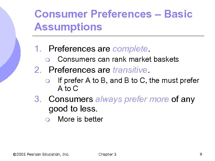
Consumer Preferences – Basic Assumptions 1. Preferences are complete. m Consumers can rank market baskets 2. Preferences are transitive. m If prefer A to B, and B to C, the must prefer A to C 3. Consumers always prefer more of any good to less. m More is better © 2005 Pearson Education, Inc. Chapter 3 9
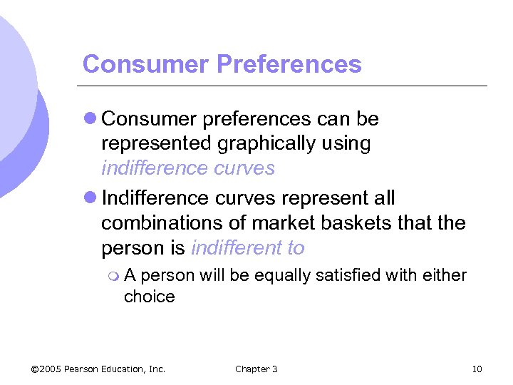
Consumer Preferences l Consumer preferences can be represented graphically using indifference curves l Indifference curves represent all combinations of market baskets that the person is indifferent to m. A person will be equally satisfied with either choice © 2005 Pearson Education, Inc. Chapter 3 10
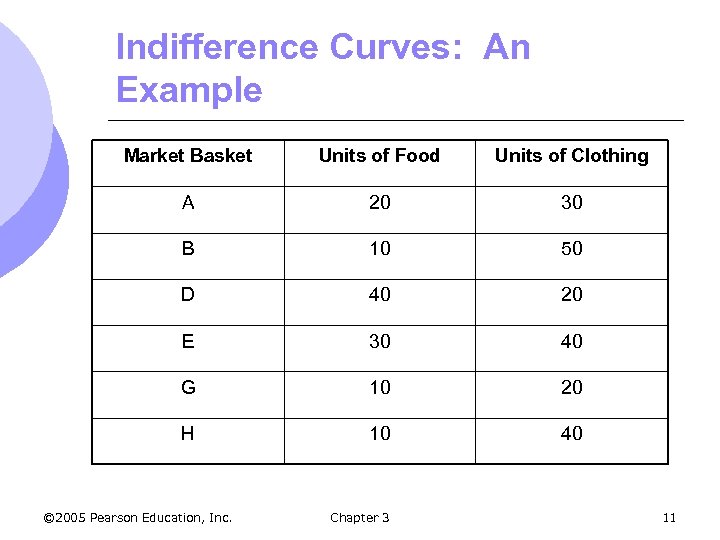
Indifference Curves: An Example Market Basket Units of Food Units of Clothing A 20 30 B 10 50 D 40 20 E 30 40 G 10 20 H 10 40 © 2005 Pearson Education, Inc. Chapter 3 11
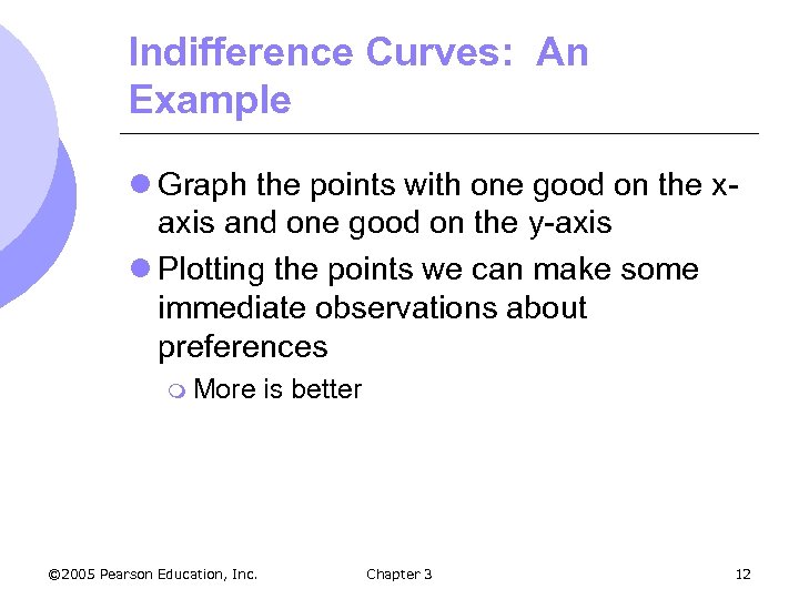
Indifference Curves: An Example l Graph the points with one good on the xaxis and one good on the y-axis l Plotting the points we can make some immediate observations about preferences m More © 2005 Pearson Education, Inc. is better Chapter 3 12
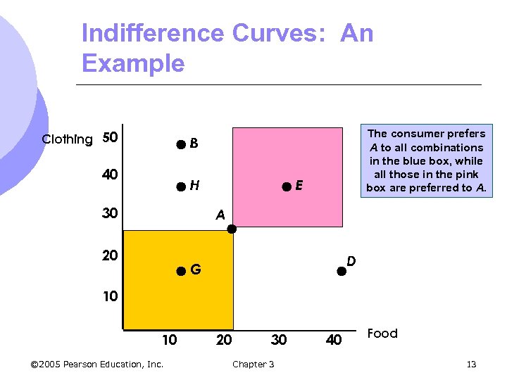
Indifference Curves: An Example Clothing 50 The consumer prefers A to all combinations in the blue box, while all those in the pink box are preferred to A. B 40 H 30 E A 20 D G 10 10 © 2005 Pearson Education, Inc. 20 30 Chapter 3 40 Food 13
Indifference Curves: An Example l Points such as B & D have more of one good but less of another compared to A m Need more information about consumer ranking l Consumer may decide they are indifference between B, A and D m We can then connect those points with an indifference curve © 2005 Pearson Education, Inc. Chapter 3 14
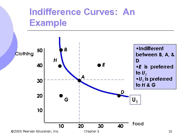
Indifference Curves: An Example Clothing 40 • Indifferent between B, A, & D • E is preferred to U 1 • U 1 is preferred to H & G B 50 H E A 30 D 20 U 1 G 10 10 © 2005 Pearson Education, Inc. 20 30 Chapter 3 40 Food 15
Indifference Curves l Any market basket lying northeast of an indifference curve is preferred to any market basket that lies on the indifference curve. l Points on the curve are preferred to points southwest of the curve © 2005 Pearson Education, Inc. Chapter 3 16
Indifference Curves l Indifference curves slope downward to the right. m If it sloped upward it would violate the assumption that more is preferred to less. l Some points that had more of both goods would be indifferent to a basket with less of both goods © 2005 Pearson Education, Inc. Chapter 3 17
Indifference Curves l To describe preferences for all combinations of goods/services, we have a set of indifference curves – an indifference map m Each indifference curve in the map shows the market baskets among which the person is indifferent. © 2005 Pearson Education, Inc. Chapter 3 18
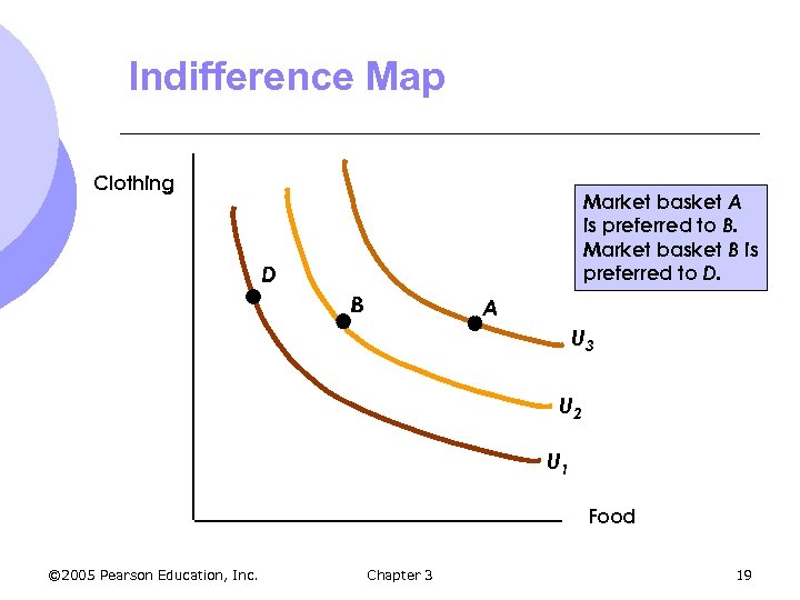
Indifference Map Clothing Market basket A is preferred to B. Market basket B is preferred to D. D B A U 3 U 2 U 1 Food © 2005 Pearson Education, Inc. Chapter 3 19
Indifference Maps l Indifference maps give more information about shapes of indifference curves m Indifference l Violates m Why? © 2005 Pearson Education, Inc. curves can not cross assumption that more is better What if we assume they can cross. Chapter 3 20
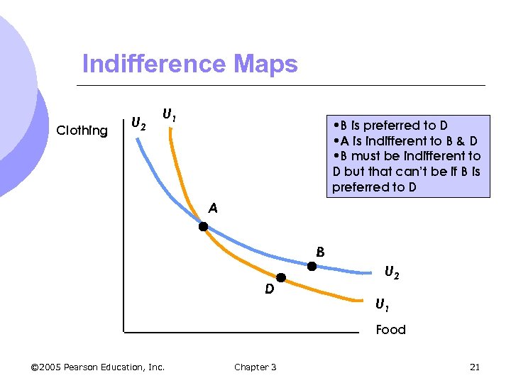
Indifference Maps Clothing U 2 U 1 • B is preferred to D • A is indifferent to B & D • B must be indifferent to D but that can’t be if B is preferred to D A B D U 2 U 1 Food © 2005 Pearson Education, Inc. Chapter 3 21
Indifference Curves l The shapes of indifference curves describes how a consumer is willing to substitute one good for another m. A to B, give up 6 clothing to get 1 food m D to E, give up 2 clothing to get 1 food l The more clothing and less food a person has, the more clothing they will give up to get more food © 2005 Pearson Education, Inc. Chapter 3 22
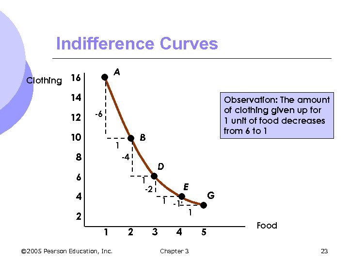
Indifference Curves A Clothing 16 14 12 Observation: The amount of clothing given up for 1 unit of food decreases from 6 to 1 -6 10 B 1 8 -4 6 D 1 -2 4 E 1 -1 2 1 © 2005 Pearson Education, Inc. 2 3 G 1 4 Chapter 3 5 Food 23
Indifference Curves l We measure how a person trades one good for another using the marginal rate of substitution (MRS) m It quantifies the amount of one good a consumer will give up to obtain more of another good. m It is measured by the slope of the indifference curve. © 2005 Pearson Education, Inc. Chapter 3 24
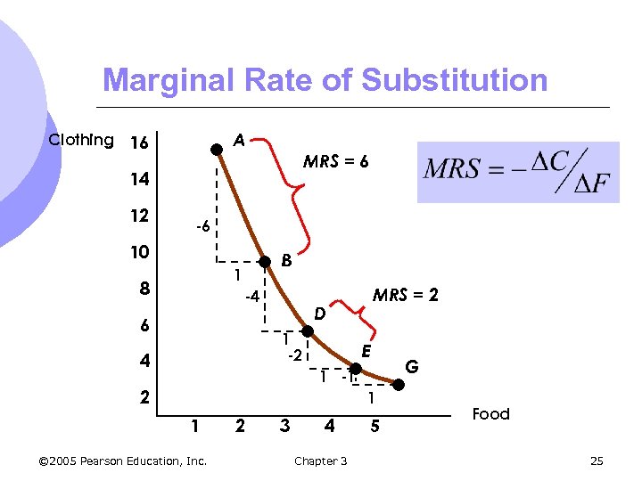
Marginal Rate of Substitution A Clothing 16 MRS = 6 14 12 -6 10 B 1 8 -4 6 D 1 -2 4 MRS = 2 E 1 -1 2 1 1 © 2005 Pearson Education, Inc. 2 3 4 Chapter 3 5 G Food 25
Marginal Rate of Substitution l Indifference curves are convex m As more of one good is consumed, a consumer would prefer to give up fewer units of a second good to get additional units of the first one. l Consumers generally prefer a balanced market basket © 2005 Pearson Education, Inc. Chapter 3 26
Marginal Rate of Substitution l The MRS decreases as we move down the indifference curve m Along an indifference curve there is a diminishing marginal rate of substitution. m The MRS went from 6 to 4 to 1 © 2005 Pearson Education, Inc. Chapter 3 27
Marginal Rate of Substitution l Indifference curves with different shapes imply a different willingness to substitute l Two polar cases are of interest m Perfect substitutes m Perfect complements © 2005 Pearson Education, Inc. Chapter 3 28
Marginal Rate of Substitution l Perfect Substitutes m Two goods are perfect substitutes when the marginal rate of substitution of one good for the other is constant. m Example: a person might consider apple juice and orange juice perfect substitutes l They would always trade 1 glass of OJ for 1 glass of Apple Juice © 2005 Pearson Education, Inc. Chapter 3 29
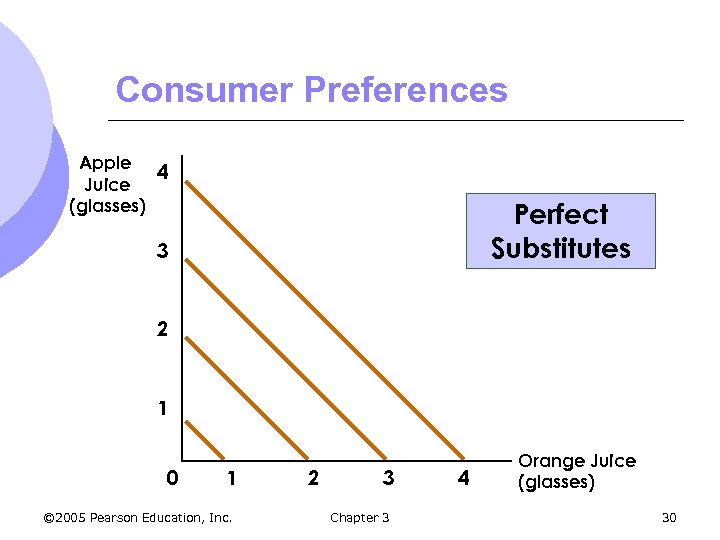
Consumer Preferences Apple 4 Juice (glasses) Perfect Substitutes 3 2 1 0 1 © 2005 Pearson Education, Inc. 2 3 Chapter 3 4 Orange Juice (glasses) 30
Consumer Preferences l Perfect Complements m Two goods are perfect complements when the indifference curves for the goods are shaped as right angles. m Example: If have 1 left shoe and 1 right shoe, you are indifferent between having more left shoes only l Must © 2005 Pearson Education, Inc. have one right for one left Chapter 3 31
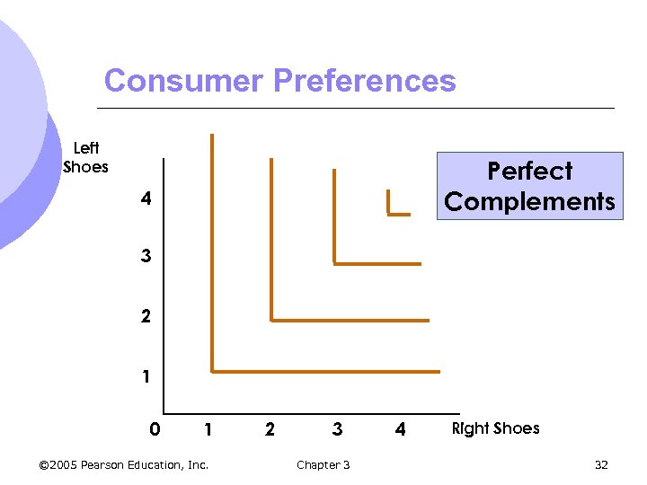
Consumer Preferences Left Shoes Perfect Complements 4 3 2 1 0 1 © 2005 Pearson Education, Inc. 2 3 Chapter 3 4 Right Shoes 32
Consumer Preferences l We have assumed all our commodities are “goods” l There are commodities we don’t want more of - bads m Things for which less is preferred to more l Examples m Air pollution m Asbestos © 2005 Pearson Education, Inc. Chapter 3 33
Consumer Preferences l How do we account for bads in our preference analysis? m We redefine the commodity l Clean air l Pollution reduction l Asbestos removal © 2005 Pearson Education, Inc. Chapter 3 34
Consumer Preferences: An Application l In designing new cars, automobile executives must determine how much time and money to invest in restyling versus increased performance m Higher demand for car with better styling and performance m Both cost more to improve © 2005 Pearson Education, Inc. Chapter 3 35
Consumer Preferences: An Application l An analysis of consumer preferences would help to determine where to spend more on change: performance or styling l Some consumers will prefer better styling and some will prefer better performance © 2005 Pearson Education, Inc. Chapter 3 36
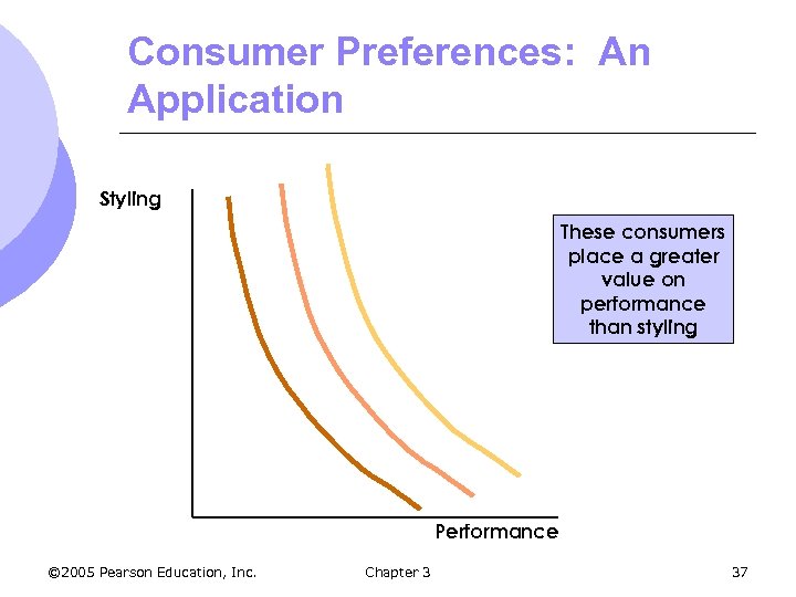
Consumer Preferences: An Application Styling These consumers place a greater value on performance than styling Performance © 2005 Pearson Education, Inc. Chapter 3 37
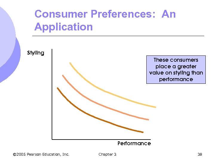
Consumer Preferences: An Application Styling These consumers place a greater value on styling than performance Performance © 2005 Pearson Education, Inc. Chapter 3 38
Consumer Preferences: An Application l Knowing which groups dominates the market will help decide where redesigning dollars should go l A recent study in the US shows that over the past two decades most consumers have preferred styling over performance. © 2005 Pearson Education, Inc. Chapter 3 39
Consumer Preferences l The theory of consumer behavior does not required assigning a numerical value to the level of satisfaction l Although ranking of market baskets are good, sometimes numerical value are useful © 2005 Pearson Education, Inc. Chapter 3 40
Consumer Preferences l Utility m. A numerical score representing the satisfaction that a consumer gets from a given market basket. m If buying 3 copies of Microeconomics makes you happier than buying one shirt, then we say that the books give you more utility than the shirt. © 2005 Pearson Education, Inc. Chapter 3 41
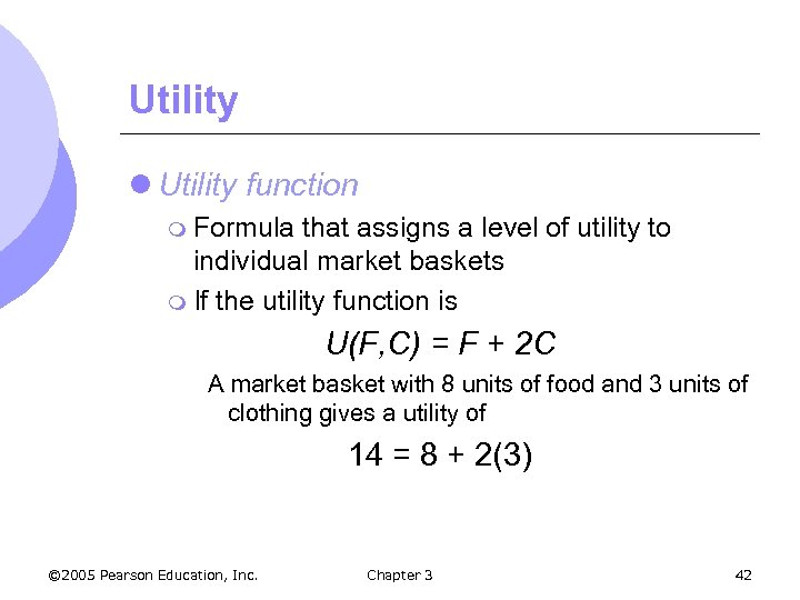
Utility l Utility function m Formula that assigns a level of utility to individual market baskets m If the utility function is U(F, C) = F + 2 C A market basket with 8 units of food and 3 units of clothing gives a utility of 14 = 8 + 2(3) © 2005 Pearson Education, Inc. Chapter 3 42
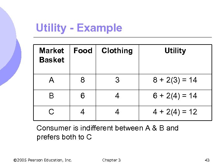
Utility - Example Market Basket Food Clothing Utility A 8 3 8 + 2(3) = 14 B 6 4 6 + 2(4) = 14 C 4 4 4 + 2(4) = 12 Consumer is indifferent between A & B and prefers both to C © 2005 Pearson Education, Inc. Chapter 3 43
Utility - Example l Baskets for each level of utility can be plotted to get an indifference curve m To find the indifference curve for a utility of 14, we can change the combinations of food and clothing that give us a utility of 14 © 2005 Pearson Education, Inc. Chapter 3 44
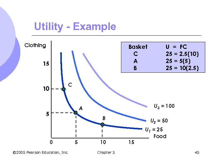
Utility - Example Clothing Basket C A B 15 U = FC 25 = 2. 5(10) 25 = 5(5) 25 = 10(2. 5) C 10 U 3 = 100 A 5 B 0 © 2005 Pearson Education, Inc. 5 10 Chapter 3 U 2 = 50 15 U 1 = 25 Food 45
Utility l Although we numerically rank baskets and indifference curves, numbers are ONLY for ranking l A utility of 4 is not necessarily twice as good as utility of 2 l There are two types of ranking m Ordinal ranking m Cardinal ranking © 2005 Pearson Education, Inc. Chapter 3 46
Utility l Ordinal Utility Function m Places market baskets in the order of most preferred to least preferred, but it does not indicate how much one market basket is preferred to another. l Cardinal Utility Function m Utility function describing the extent to which one market basket is preferred to another. © 2005 Pearson Education, Inc. Chapter 3 47
Utility l The actual unit of measurement for utility is not important. l An ordinal ranking is sufficient to explain how most individual decisions are made. © 2005 Pearson Education, Inc. Chapter 3 48
Budget Constraints l Preferences do not explain all of consumer behavior. l Budget constraints also limit an individual’s ability to consume in light of the prices they must pay for various goods and services. © 2005 Pearson Education, Inc. Chapter 3 49
Budget Constraints l The Budget Line m Indicates all combinations of two commodities for which total money spent equals total income. m We assume only 2 goods are consumed, so we do not consider savings © 2005 Pearson Education, Inc. Chapter 3 50
The Budget Line l Let F equal the amount of food purchased, and C is the amount of clothing. l Price of food = PF and price of clothing = PC l Then PF F is the amount of money spent on food, and PC C is the amount of money spent on clothing. © 2005 Pearson Education, Inc. Chapter 3 51
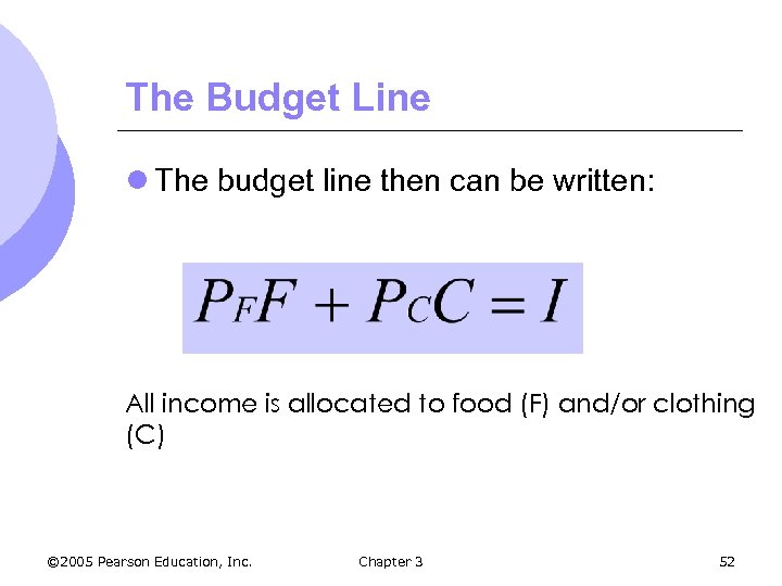
The Budget Line l The budget line then can be written: All income is allocated to food (F) and/or clothing (C) © 2005 Pearson Education, Inc. Chapter 3 52
The Budget Line l Different choices of food and clothing can be calculated that use all income m These choices can be graphed as the budget line l Example: m Assume = $2 © 2005 Pearson Education, Inc. income of $80/week, PF = $1 and PC Chapter 3 53
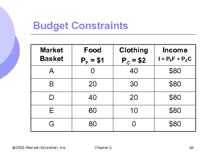
Budget Constraints Market Basket Clothing PC = $2 40 I = PFF + PCC A Food PF = $1 0 B 20 30 $80 D 40 20 $80 E 60 10 $80 G 80 0 $80 © 2005 Pearson Education, Inc. Chapter 3 Income $80 54
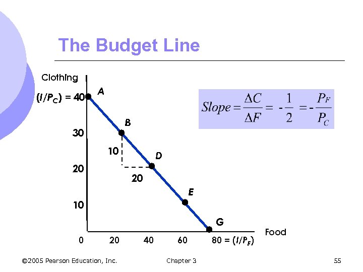
The Budget Line Clothing (I/PC) = 40 A B 30 10 20 D 20 E 10 G 0 20 © 2005 Pearson Education, Inc. 40 60 Chapter 3 80 = (I/PF) Food 55
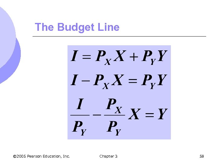
The Budget Line l As consumption moves along a budget line from the intercept, the consumer spends less on one item and more on the other. l The slope of the line measures the relative cost of food and clothing. l The slope is the negative of the ratio of the prices of the two goods. © 2005 Pearson Education, Inc. Chapter 3 56
The Budget Line l The slope indicates the rate at which the two goods can be substituted without changing the amount of money spent. l We can rearrange the budget line equation to make this more clear © 2005 Pearson Education, Inc. Chapter 3 57
The Budget Line © 2005 Pearson Education, Inc. Chapter 3 58
Budget Constraints l The Budget Line m The vertical intercept (I/PC), illustrates the maximum amount of C that can be purchased with income I. m The horizontal intercept (I/PF), illustrates the maximum amount of F that can be purchased with income I. © 2005 Pearson Education, Inc. Chapter 3 59
The Budget Line l As we know, income and prices can change l As incomes and prices change, there are changes in budget lines l We can show the effects of these changes on budget lines and consumer choices © 2005 Pearson Education, Inc. Chapter 3 60
The Budget Line - Changes l The Effects of Changes in Income m An increase in income causes the budget line to shift outward, parallel to the original line (holding prices constant). m Can buy more of both goods with more income © 2005 Pearson Education, Inc. Chapter 3 61
The Budget Line - Changes l The Effects of Changes in Income m. A decrease in income causes the budget line to shift inward, parallel to the original line (holding prices constant). m Can buy less of both goods with less income © 2005 Pearson Education, Inc. Chapter 3 62
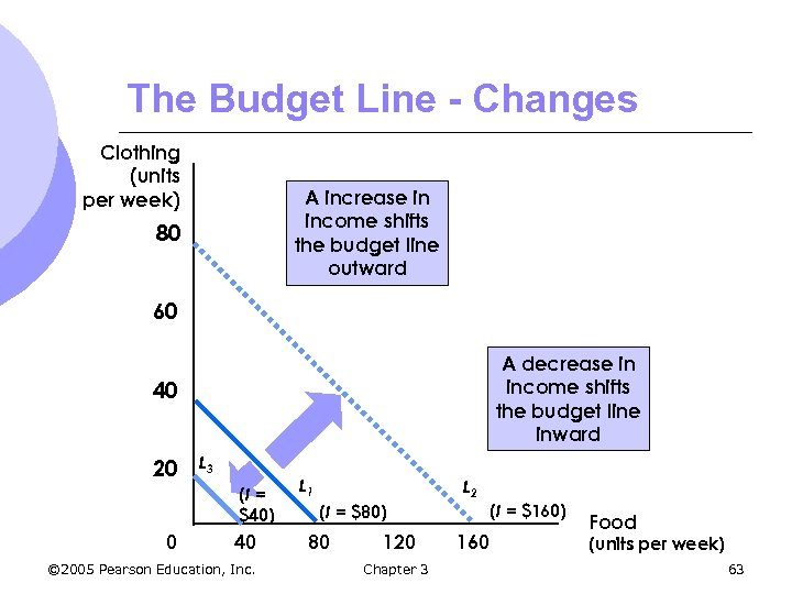
The Budget Line - Changes Clothing (units per week) A increase in income shifts the budget line outward 80 60 A decrease in income shifts the budget line inward 40 20 L 3 (I = $40) 0 40 © 2005 Pearson Education, Inc. L 1 L 2 (I = $80) 80 120 Chapter 3 (I = $160) 160 Food (units per week) 63
The Budget Line - Changes l The Effects of Changes in Prices m If the price of one good increases, the budget line shifts inward, pivoting from the other good’s intercept. m If price of food increases and you buy only food (x-intercept), then can’t buy as much food. The point shifts in m If buy only clothing (y-intercept), can buy the same amount. No change © 2005 Pearson Education, Inc. Chapter 3 64
The Budget Line - Changes l The Effects of Changes in Prices m If the price of one good decreases, the budget line shifts outward, pivoting from the other good’s intercept. m If price of food decreases and you buy only food (x-intercept), then can buy more food. The point shifts out. m If buy only clothing (y-intercept), can buy the same amount. No change © 2005 Pearson Education, Inc. Chapter 3 65
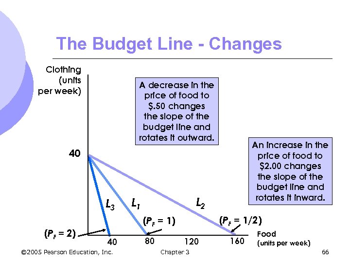
The Budget Line - Changes Clothing (units per week) A decrease in the price of food to $. 50 changes the slope of the budget line and rotates it outward. An increase in the price of food to $2. 00 changes the slope of the budget line and rotates it inward. 40 L 3 (PF = 2) L 2 L 1 (PF = 1/2) (PF = 1) 40 © 2005 Pearson Education, Inc. 80 120 Chapter 3 160 Food (units per week) 66
The Budget Line - Changes l The Effects of Changes in Prices m If the two goods increase in price, but the ratio of the two prices is unchanged, the slope will not change. m However, the budget line will shift inward to a point parallel to the original budget line © 2005 Pearson Education, Inc. Chapter 3 67
The Budget Line - Changes l The Effects of Changes in Prices m If the two goods decrease in price, but the ratio of the two prices is unchanged, the slope will not change. m However, the budget line will shift outward to a point parallel to the original budget line © 2005 Pearson Education, Inc. Chapter 3 68
Consumer Choice l Given preferences and budget constraints, how do consumers choose what to buy? l Consumers choose a combination of goods that will maximize their satisfaction, given the limited budget available to them. © 2005 Pearson Education, Inc. Chapter 3 69
Consumer Choice l The maximizing market basket must satisfy two conditions: 1. It must be located on the budget line. m They spend all their income – more is better 2. It must give the consumer the most preferred combination of goods and services. © 2005 Pearson Education, Inc. Chapter 3 70
Consumer Choice l Graphically we can see different indifference curves of a consumer choosing between clothing and food l Remember that U 3 > U 2 > U 1 for our indifference curves l Consumer wants to choose highest utility within their budget © 2005 Pearson Education, Inc. Chapter 3 71
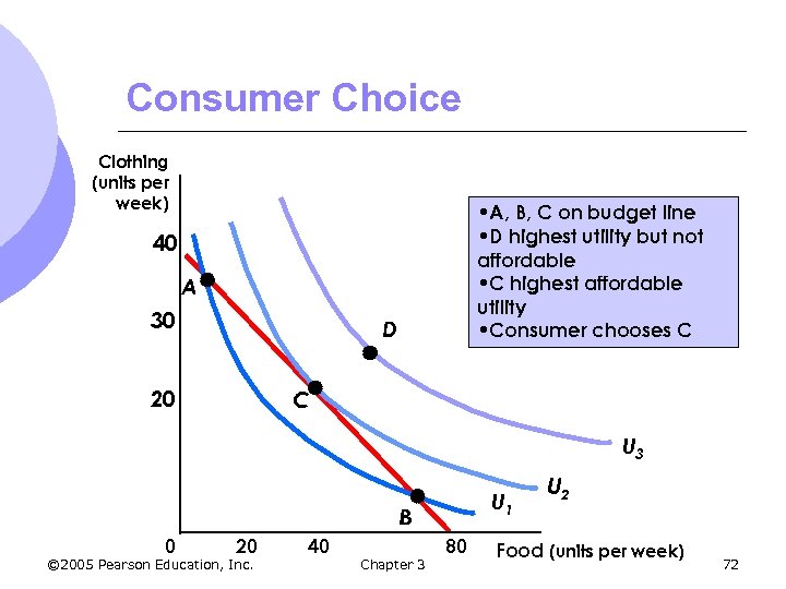
Consumer Choice Clothing (units per week) • A, B, C on budget line • D highest utility but not affordable • C highest affordable utility • Consumer chooses C 40 A 30 D 20 C U 3 U 1 B 0 20 © 2005 Pearson Education, Inc. 40 Chapter 3 80 U 2 Food (units per week) 72
Consumer Choice l Consumer will choose highest indifference curve on budget line l In previous graph, point C is where the indifference curve is just tangent to the budget line l Slope of the budget line equals the slope of the indifference curve at this point © 2005 Pearson Education, Inc. Chapter 3 73
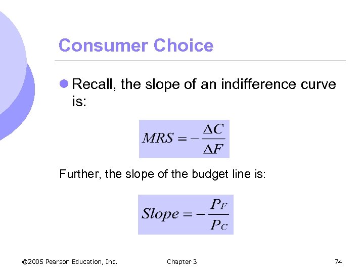
Consumer Choice l Recall, the slope of an indifference curve is: Further, the slope of the budget line is: © 2005 Pearson Education, Inc. Chapter 3 74
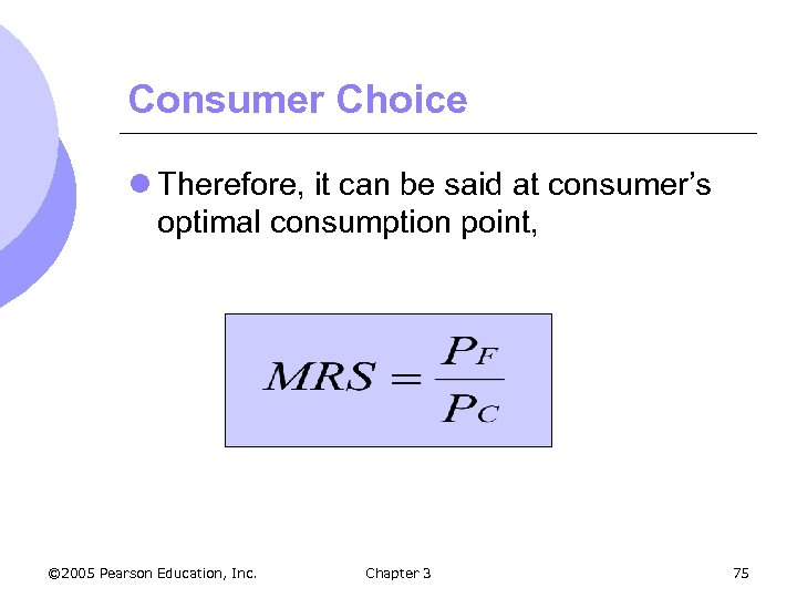
Consumer Choice l Therefore, it can be said at consumer’s optimal consumption point, © 2005 Pearson Education, Inc. Chapter 3 75
Consumer Choice l It can be said that satisfaction is maximized when marginal rate of substitution (of F and C) is equal to the ratio of the prices (of F and C). l Note this is ONLY true at the optimal consumption point © 2005 Pearson Education, Inc. Chapter 3 76
Consumer Choice l Optimal consumption point is where marginal benefits equal marginal costs l MB = MRS = benefit associated with consumption of 1 more unit of food l MC = cost of additional unit of food m 1 unit food = ½ unit clothing m PF/PC © 2005 Pearson Education, Inc. Chapter 3 77
Consumer Choice l If MRS ≠ PF/PC then individuals can reallocate basket to increase utility l If MRS > PF/PC m Will increase food and decrease clothing until MRS = PF/PC l If MRS < PF/PC m Will increase clothing and decrease food until MRS = PF/PC © 2005 Pearson Education, Inc. Chapter 3 78
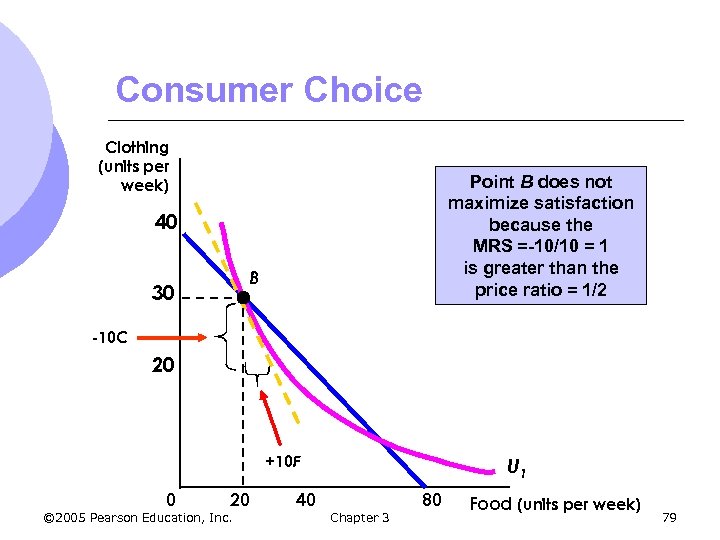
Consumer Choice Clothing (units per week) Point B does not maximize satisfaction because the MRS =-10/10 = 1 is greater than the price ratio = 1/2 40 B 30 -10 C 20 +10 F 0 20 © 2005 Pearson Education, Inc. 40 U 1 Chapter 3 80 Food (units per week) 79
Consumer Choice: An Application Revisited l Consider two groups of consumers, each wishing to spend $10, 000 on the styling and performance of a car. l Each group has different preferences. © 2005 Pearson Education, Inc. Chapter 3 80
Consumer Choice: An Application Revisited l By finding the point of tangency between a group’s indifference curve and the budget constraint auto companies can see how much consumers value each attribute. © 2005 Pearson Education, Inc. Chapter 3 81
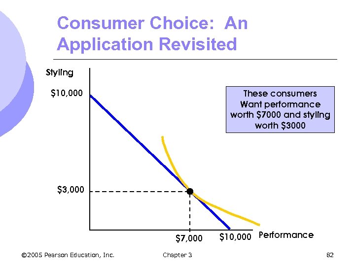
Consumer Choice: An Application Revisited Styling $10, 000 These consumers Want performance worth $7000 and styling worth $3000 $3, 000 $7, 000 © 2005 Pearson Education, Inc. Chapter 3 $10, 000 Performance 82
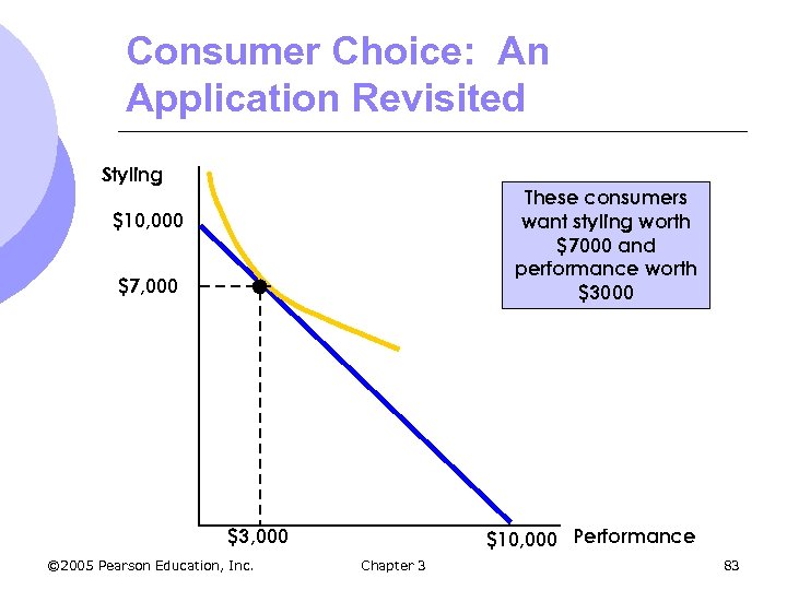
Consumer Choice: An Application Revisited Styling These consumers want styling worth $7000 and performance worth $3000 $10, 000 $7, 000 $10, 000 Performance $3, 000 © 2005 Pearson Education, Inc. Chapter 3 83
Consumer Choice: An Application Revisited l Once know preferences, can design a production and marketing plan l Company can then make a sensible strategic business decision on how to allocate performance and styling on new cars © 2005 Pearson Education, Inc. Chapter 3 84
Consumer Choice l A corner solution exists if a consumer buys in extremes, and buys all of one category of good and none of another. m MRS © 2005 Pearson Education, Inc. is not necessarily equal to PA/PB Chapter 3 85
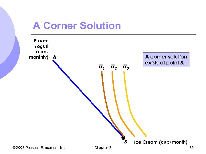
A Corner Solution Frozen Yogurt (cups monthly) A U 1 U 2 U 3 B © 2005 Pearson Education, Inc. Chapter 3 A corner solution exists at point B. Ice Cream (cup/month) 86
A Corner Solution l At point B, the MRS of ice cream for frozen yogurt is greater than the slope of the budget line. l f the consumer could give up more frozen yogurt for ice cream he would do so. l However, there is no more frozen yogurt to give up l Opposite is true if corner solution was at point A © 2005 Pearson Education, Inc. Chapter 3 87
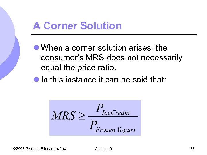
A Corner Solution l When a corner solution arises, the consumer’s MRS does not necessarily equal the price ratio. l In this instance it can be said that: © 2005 Pearson Education, Inc. Chapter 3 88
A Corner Solution l If the MRS is, in fact, significantly greater than the price ratio, then a small decrease in the price of frozen yogurt will not alter the consumer’s market basket. © 2005 Pearson Education, Inc. Chapter 3 89
A Corner Solution - Example l Suppose Jane Doe’s parents set up a trust fund for her college education. l The money must be used only for education. l Although a welcome gift, an unrestricted gift might be better © 2005 Pearson Education, Inc. Chapter 3 90
A Corner Solution - Example l Original budget line, PQ, with a market basket, A, of education and other goods l Trust fund shifts out the budget line as long as trust fund, PB, spent on education l Jane increases satisfaction moving to higher indifference curve, U 2 © 2005 Pearson Education, Inc. Chapter 3 91
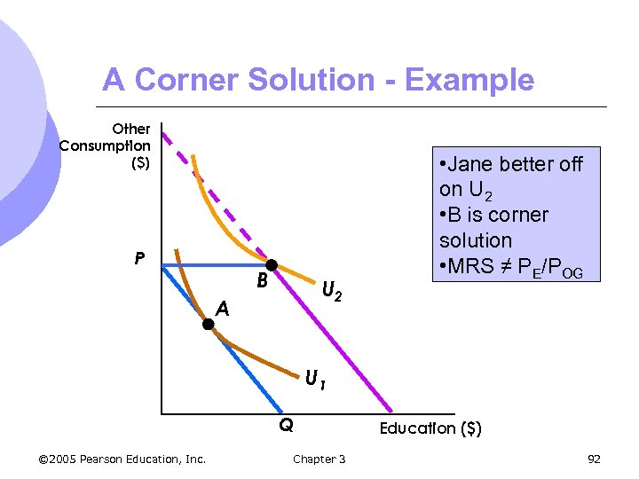
A Corner Solution - Example Other Consumption ($) P B U 2 A • Jane better off on U 2 • B is corner solution • MRS ≠ PE/POG U 1 Q © 2005 Pearson Education, Inc. Chapter 3 Education ($) 92
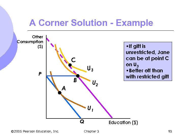
A Corner Solution - Example Other Consumption ($) C U 3 P B U 2 A • If gift is unrestricted, Jane can be at point C on U 3 • Better off than with restricted gift U 1 Q © 2005 Pearson Education, Inc. Chapter 3 Education ($) 93
Revealed Preferences l If we know the choices a consumer has made, we can determine what their preferences are if we have information about a sufficient number of choices that are made when prices and incomes vary. © 2005 Pearson Education, Inc. Chapter 3 94
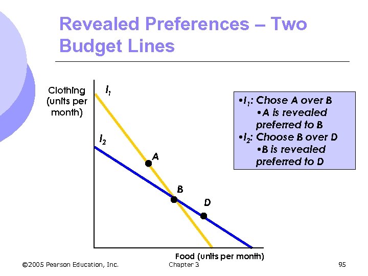
Revealed Preferences – Two Budget Lines Clothing (units per month) l 1 • I 1: Chose A over B • A is revealed preferred to B • l 2: Choose B over D • B is revealed preferred to D l 2 A B D © 2005 Pearson Education, Inc. Food (units per month) Chapter 3 95
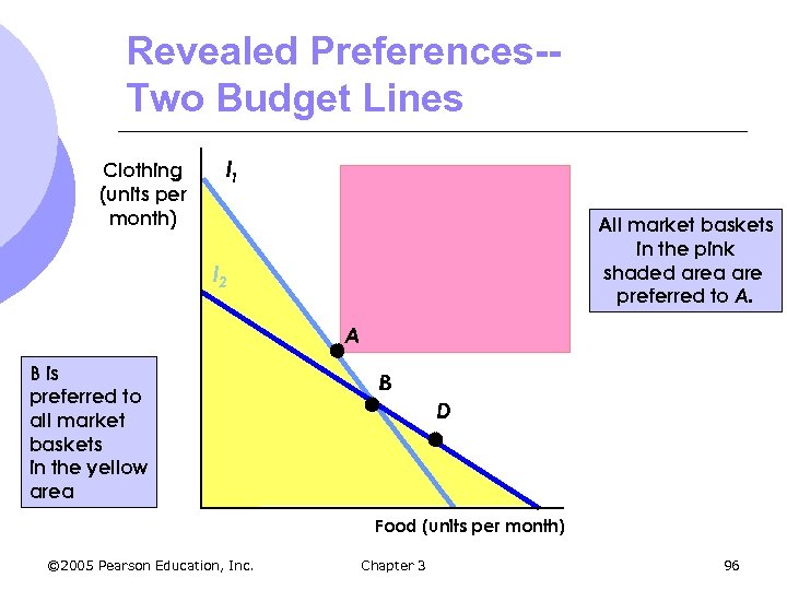
Revealed Preferences-Two Budget Lines Clothing (units per month) l 1 All market baskets in the pink shaded area are preferred to A. l 2 A B is preferred to all market baskets in the yellow area B D Food (units per month) © 2005 Pearson Education, Inc. Chapter 3 96
Revealed Preference l As you continue to change the budget line, individuals can tell you which basket they prefer to others. l More the individual reveals, the more you can discern about their preferences l Eventually you can map out an indifference curve © 2005 Pearson Education, Inc. Chapter 3 97
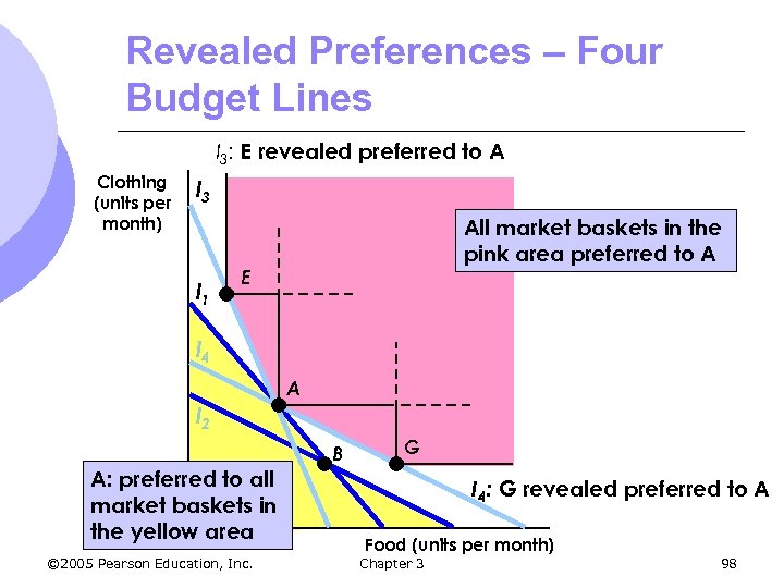
Revealed Preferences – Four Budget Lines I 3: E revealed preferred to A Clothing (units per month) l 3 l 1 All market baskets in the pink area preferred to A E l 4 A l 2 B A: preferred to all market baskets in the yellow area © 2005 Pearson Education, Inc. G I 4: G revealed preferred to A Food (units per month) Chapter 3 98
Marginal Utility and Consumer Choice l Marginal utility measures the additional satisfaction obtained from consuming one additional unit of a good. m How much happier is the individual from consuming one more unit of food © 2005 Pearson Education, Inc. Chapter 3 99
Marginal Utility - Example l The marginal utility derived from increasing from 0 to 1 units of food might be 9 l Increasing from 1 to 2 might be 7 l Increasing from 2 to 3 might be 5 l Observation: Marginal utility is diminishing as consumption increases © 2005 Pearson Education, Inc. Chapter 3 100
Marginal Utility l The principle of diminishing marginal utility states that as more of a good is consumed, the additional utility the consumer gains will be smaller and smaller. l Note that total utility will continue to increase since consumer makes choices that make them happier © 2005 Pearson Education, Inc. Chapter 3 101
Marginal Utility and Indifference Curves l As consumption moves along an indifference curve: m Additional utility derived from an increase in the consumption one good, food (F), must balance the loss of utility from the decrease in the consumption in the other good, clothing (C). © 2005 Pearson Education, Inc. Chapter 3 102
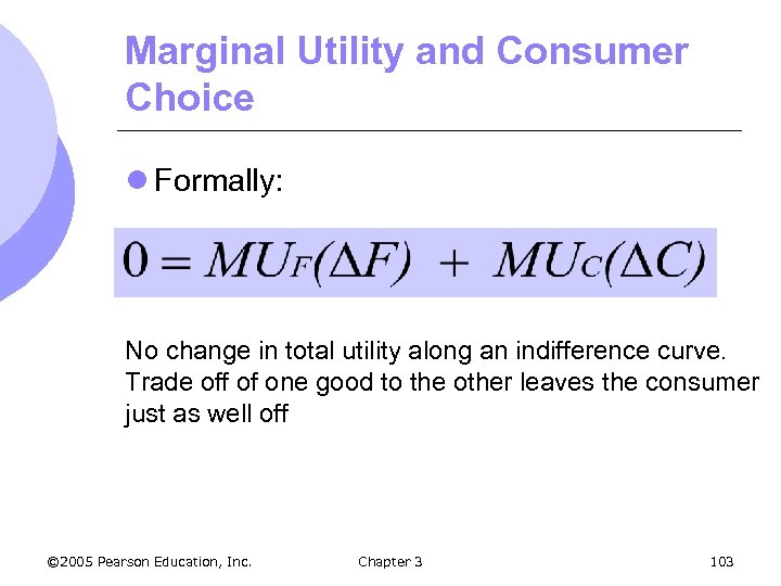
Marginal Utility and Consumer Choice l Formally: No change in total utility along an indifference curve. Trade off of one good to the other leaves the consumer just as well off © 2005 Pearson Education, Inc. Chapter 3 103
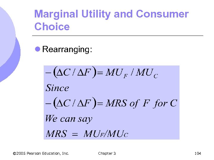
Marginal Utility and Consumer Choice l Rearranging: © 2005 Pearson Education, Inc. Chapter 3 104
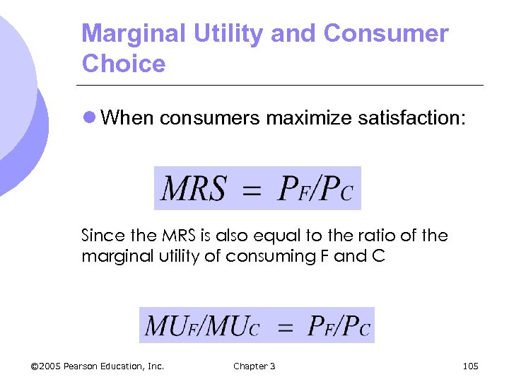
Marginal Utility and Consumer Choice l When consumers maximize satisfaction: Since the MRS is also equal to the ratio of the marginal utility of consuming F and C © 2005 Pearson Education, Inc. Chapter 3 105
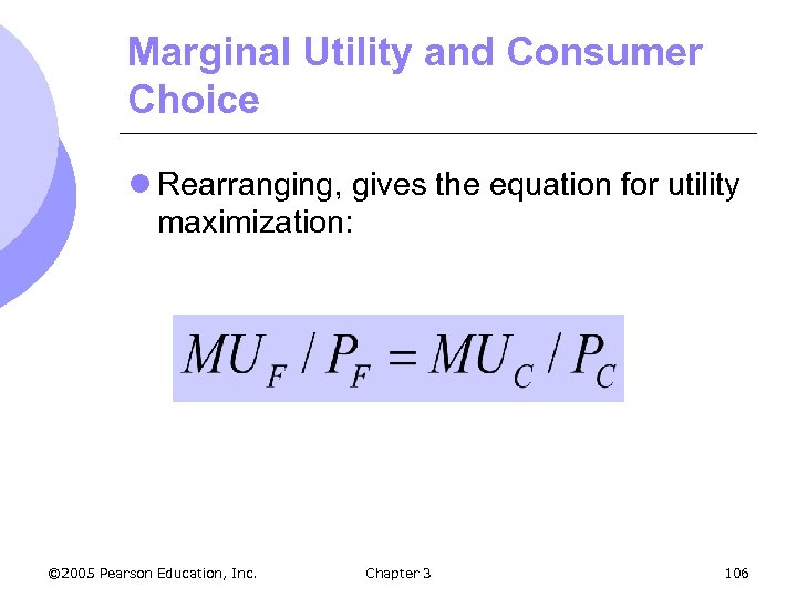
Marginal Utility and Consumer Choice l Rearranging, gives the equation for utility maximization: © 2005 Pearson Education, Inc. Chapter 3 106
Marginal Utility and Consumer Choice l Total utility is maximized when the budget is allocated so that the marginal utility per dollar of expenditure is the same for each good. l This is referred to as the equal marginal principle. © 2005 Pearson Education, Inc. Chapter 3 107
Cost-of-Living Indexes l Social security payments are given to qualifying individuals l Each year the benefit increases equal to the rate of increase of the Consumer Price Index (CPI) m Ratio of the present cost of typical bundle of goods/services in comparison to the cost during a base period © 2005 Pearson Education, Inc. Chapter 3 108
Cost-of-Living Indexes l Does the CPI give a good measure of inflation and therefore a measure of the cost of living changes? l Should the CPI be used to measure how much cost of living has increased determining increases in government payment programs? © 2005 Pearson Education, Inc. Chapter 3 109
Cost-of-Living Indexes l The ideal cost of living index represents the cost of attaining a given level of utility at current prices relative to the cost of attaining the same utility at base prices © 2005 Pearson Education, Inc. Chapter 3 110
Cost-of-Living Indexes l To obtain the ideal cost of living index would require too much information such as consumer preferences as well as prices and expenditures l Actual price indexes are based on consumer purchases, not preferences © 2005 Pearson Education, Inc. Chapter 3 111
Cost-of-Living Indexes l Laspeyres price index m Amount of money at current year prices that an individual requires to purchase a bundle of goods/services chosen in a base year divided by the cost of purchasing the same bundle at base-year prices m Ex: CPI © 2005 Pearson Education, Inc. Chapter 3 112
Cost-of-Living Indexes l The Laspeyres price index assumes that consumers do not alter their consumption patterns as prices change l Tend to overstate the true cost of living index l Using the CPI to adjust retirement benefits will tend to overcompensate most recipients requiring greater government expenditure © 2005 Pearson Education, Inc. Chapter 3 113
Cost-of-Living Indexes l Paasche index m Focuses on the cost of buying the current year’s bundle m Amount of money at current –year prices that an individual requires to purchase a current bundle of goods/services divided by the cost of purchasing the same bundle in a base year © 2005 Pearson Education, Inc. Chapter 3 114
Cost-of-Living Indexes l Comparison of indexes m Both are fixed weight indexes m Quantities of various goods and services in each index remain unchanged m Laspeyres index keeps quantities at base year levels m Paasche index keeps unchanged quantities at current year levels © 2005 Pearson Education, Inc. Chapter 3 115
Cost-of-Living Indexes l Chain-Weighted Indexes m Cost-of-living index that accounts for changes in quantities of goods and services m Introduced to overcome problems that arose when long-term comparisons were make using fixed weight price indexes © 2005 Pearson Education, Inc. Chapter 3 116
597553a3c6bffa4b827dc355b17fcc2a.ppt