6443924b9d6c3ae8a8931853ff9874ea.ppt
- Количество слайдов: 93
 Chapter 3 Applications of Linear and Integer Programming Models - 1 1
 3. 1 The Evolution of Linear Programming Models in Business and Government • Many examples are presented that demonstrate the successful application of linear and integer programming. • Our goals are to: – Examine potential application areas – Develop good modeling skills – Illustrate the use of spreadsheets to generate results – Interpret properly and analyze spreadsheet results 2
 Examples of Linear Programming Models in Business and Government • • • An optimal portfolio Optimal scheduling of personnel An optimal blend of raw crude oils A minimized cost diet An operation and shipping pattern The optimal production levels 3
 Examples of Linear Programming Models in Business and Government • The optimal assignment of fleets to flights • How to best expand a communication network • An efficient air-pollution control system • An agricultural resource allocation plan • The set of public projects to select 4
 3. 2 Building Good Linear and Integer Programming Models • Three important factors may affect the successful process of building good models: – Familiarity – Simplicity – Clarity 5
 – Begin by listing the details of the problem in short phrases. – Determine the objective in general terms and then determine what is within the control of the decision maker (decision variables). – Add decision variables as needed during the course of formulation to accurately express objective function and constraints. – Define the decision variables precisely. 6
 Summation Variables / Constraints • Many times the use of summation variables (representing the sum of all or of part of the decision variables) along with the summation constraints associated with them, may simplify models’ formulation. • See the following example. 7
 Summation Variables / Constraints • Example – Three television models are to be produced. – Each model uses 2, 3, and 4 pounds of plastic respectively. – 7000 pounds of plastic are available. – No model should exceed 40% of the total quantity produced. – The profit per set is $23, $34, and $45 respectively. – Find the production plan that maximizes the 8 profit.
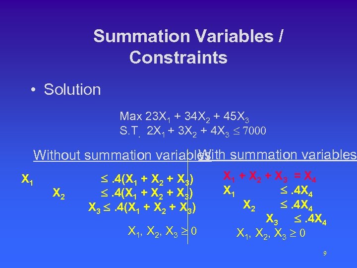 Summation Variables / Constraints • Solution Max 23 X 1 + 34 X 2 + 45 X 3 S. T. 2 X 1 + 3 X 2 + 4 X 3 £ 7000 Without summation variables X 1 X 2 . 4(X 1 + X 2 + X 3) X 3 . 4(X 1 + X 2 + X 3) X 1, X 2, X 3 ³ 0 X 1 + X 2 + X 3 = X 4 X 1 . 4 X 4 X 2 . 4 X 4 X 3 . 4 X 4 X 1, X 2, X 3 ³ 0 9
 A checklist for building linear models – Formulate a relationship / function in words before formulating it in mathematical terms. (Expression) [Has some relation to] (Another+10 A + 2 B 2 A + B expression or constant) – Bring the expression to the form: (Expression) [Relation] (Constant) -A +B £ ³ 10 10
 A checklist for building linear models – Keep the units on both sides of the expressions consistent – Use summation variables when appropriate – Indicate which variables are § Non-negative § Integers § Binary 11
 • Additional variables / constraints – Use definitional variables to simplify problem formulation (particularly useful in “percentage” constraints. ) – Specify variables with the following restrictions: • Non-negativity. • Upper and lower bound. • Integrality. 12
 3. 4 Applications of Linear Programming Models • The modeling of real problems is illustrated in this section. • Examples include: – – Production Purchasing Finance Cash flow accounting 13
 3. 4 Applications of Linear Programming Models • The modeling of real problems is illustrated in this section. • Examples include: – – Production Purchasing Finance Cash flow accounting • Emphasis is given to: – Various application area, – Model development, – Spreadsheet design, – Analysis and interpretation of the output. 14
 3. 4. 1 Production Scheduling Models • These models can assist managers in making decision regarding the efficient utilization of scarce resource. • Applications include: – Determining production levels – Scheduling shifts – Using overtime – The cost effectiveness of adding resources 15
 Galaxy Industries Expansion Plan • Galaxy Industries is planning to increase its production and include two new products • Data – Up to 3000 pounds of plastic will be available. – Regular time available will be 40 hours. – Overtime available will be 32 hours. – One hour of overtime costs $180 more than one hour of regular time. 16
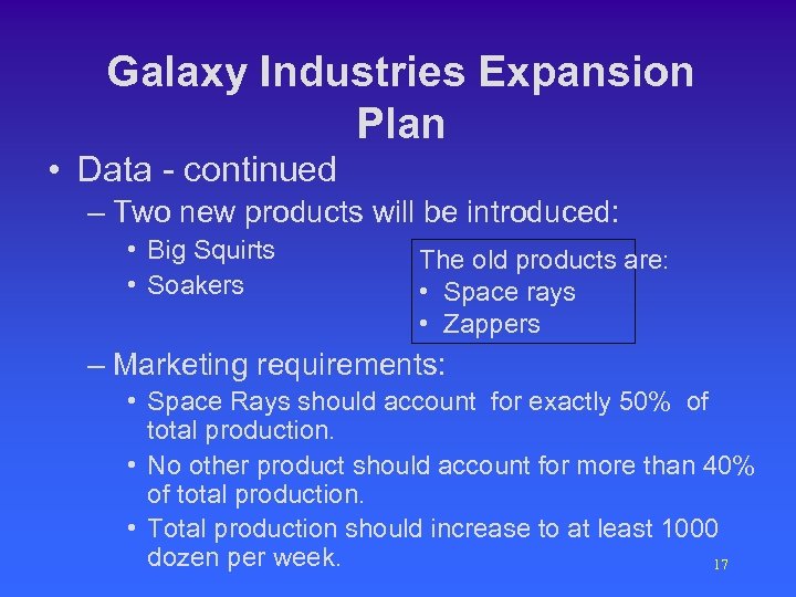 Galaxy Industries Expansion Plan • Data - continued – Two new products will be introduced: • Big Squirts • Soakers The old products are: • Space rays • Zappers – Marketing requirements: • Space Rays should account for exactly 50% of total production. • No other product should account for more than 40% of total production. • Total production should increase to at least 1000 dozen per week. 17
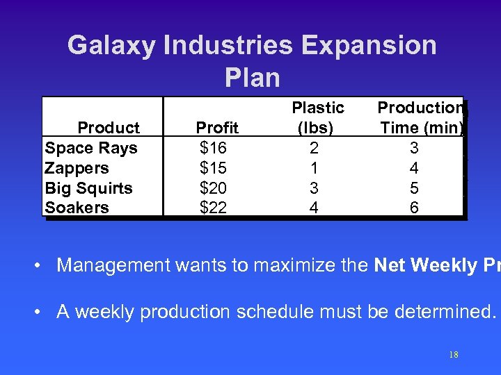 Galaxy Industries Expansion Plan • Data - Continued Product Space Rays Zappers Big Squirts Soakers Profit $16 $15 $20 $22 Plastic (lbs) 2 2 1 1 3 3 4 4 Production Time (min) 3 3 4 4 5 5 6 6 • Management wants to maximize the Net Weekly Pr • A weekly production schedule must be determined. 18
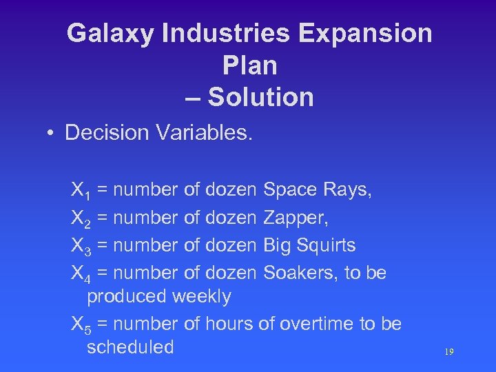 Galaxy Industries Expansion Plan – Solution • Decision Variables. X 1 = number of dozen Space Rays, X 2 = number of dozen Zapper, X 3 = number of dozen Big Squirts X 4 = number of dozen Soakers, to be produced weekly X 5 = number of hours of overtime to be scheduled 19
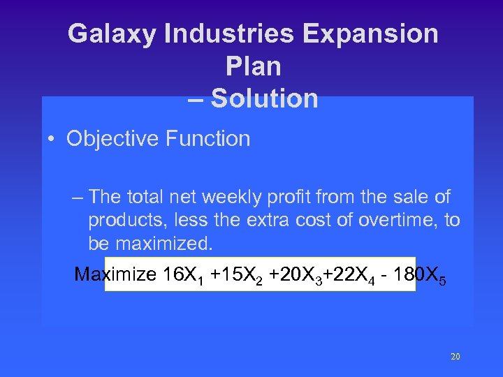 Galaxy Industries Expansion Plan – Solution • Objective Function – The total net weekly profit from the sale of products, less the extra cost of overtime, to be maximized. Maximize 16 X 1 +15 X 2 +20 X 3+22 X 4 - 180 X 5 20
 Galaxy Industries Expansion Plan – Solution • Constraints 21
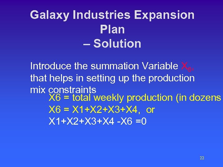 Galaxy Industries Expansion Plan – Solution Introduce the summation Variable X 6, that helps in setting up the production mix constraints X 6 = total weekly production (in dozens X 6 = X 1+X 2+X 3+X 4, or X 1+X 2+X 3+X 4 -X 6 =0 22
 Galaxy Industries Expansion Plan 23
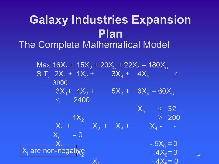 Galaxy Industries Expansion Plan The Complete Mathematical Model Max 16 X 1 + 15 X 2 + 20 X 3 + 22 X 4 – 180 X 5 S. T. 2 X 1 + 1 X 2 + 3 X 3 + 4 X 4 £ 3000 3 X 1+ 4 X 2 + 5 X 3 + 6 X 4 – 60 X 5 £ 2400 X 5 £ 32 1 X 2 ³ 200 X 1 + X 2 + X 3 + X 4 X 6 =0 X 1 -. 5 X 6 = 0 Xj are non-negative X 2 -. 4 X 6 = 0 X -. 4 X = 0 24
 25
25
 26
26
 27
27
 28
28
 29
29
 30
30
 31
31
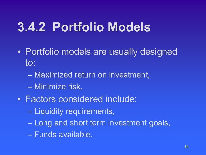 3. 4. 2 Portfolio Models • Portfolio models are usually designed to: – Maximized return on investment, – Minimize risk. • Factors considered include: – Liquidity requirements, – Long and short term investment goals, – Funds available. 34
 Jones Investment • Charles’ Evaluation 35
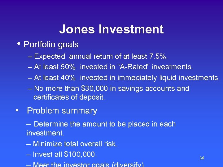 Jones Investment • Portfolio goals – Expected annual return of at least 7. 5%. – At least 50% invested in “A-Rated” investments. – At least 40% invested in immediately liquid investments. – No more than $30, 000 in savings accounts and certificates of deposit. • Problem summary – Determine the amount to be placed in each investment. – Minimize total overall risk. – Invest all $100, 000. 36
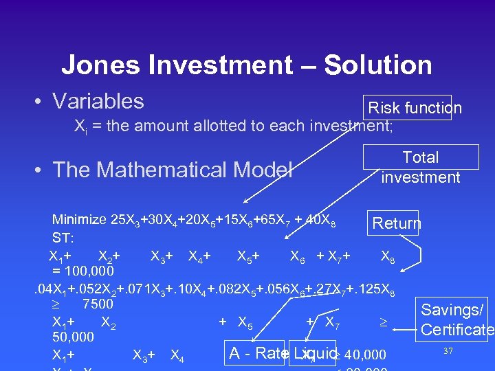 Jones Investment – Solution • Variables Risk function Xi = the amount allotted to each investment; • The Mathematical Model Total investment Minimize 25 X 3+30 X 4+20 X 5+15 X 6+65 X 7 + 40 X 8 Return ST: X 1+ X 2+ X 3+ X 4+ X 5+ X 6 + X 7+ X 8 = 100, 000. 04 X 1+. 052 X 2+. 071 X 3+. 10 X 4+. 082 X 5+. 056 X 6+. 27 X 7+. 125 X 8 ³ 7500 Savings/ X 1 + X 2 + X 5 + X 7 ³ Certificate 50, 000 37 A - Rate Liquid 40, 000 X 1 + X 3 + X 4 + X 7 ³
 38
38
 39
39
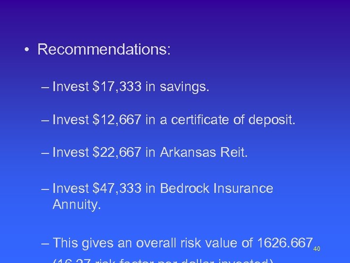 • Recommendations: – Invest $17, 333 in savings. – Invest $12, 667 in a certificate of deposit. – Invest $22, 667 in Arkansas Reit. – Invest $47, 333 in Bedrock Insurance Annuity. – This gives an overall risk value of 1626. 66740
 41
41
 42
42
 43
43
 44
44
 3. 4. 3 Public Sector Models • Governments in the public sector are charged with distributing resources for the public good. • The public good can be measured by – Traditional objectives (i. e. cost minimization), – Specific functions developed to measure the public satisfaction or preference. • The constraints represent (among others) – Resource availability, – Social issues (diversity, equality) 45
 St. Joseph Inspection Problem • St. Joseph Public Utility Commission needs to inspect and report utility problems in a flood area. Experts are assigned to inspect: • Homes • Offices • Plants Three types of inspection will be conducted: • Electrical • Gas • Insulation 46
 St. Joseph Inspection Problem • Problem Summary – St. Joseph Public Utility Commission needs to determine the number of homes, office complexes, and plants to be inspected. – The objective is to maximize the total number of structures inspected, under certain requirements. 47
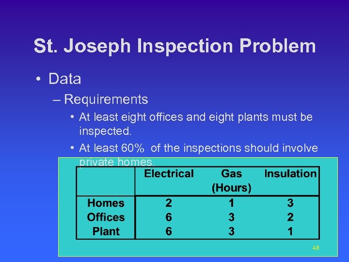 St. Joseph Inspection Problem • Data – Requirements • At least eight offices and eight plants must be inspected. • At least 60% of the inspections should involve private homes. 48
 St. Joseph Inspection Problem • Data – Resources • At most, 120 hours can be allocated for electrical inspections. • At most 80 hours can be allocated for gas inspection. • At most 100 consulting hours can be allocated for insulation inspection. 49
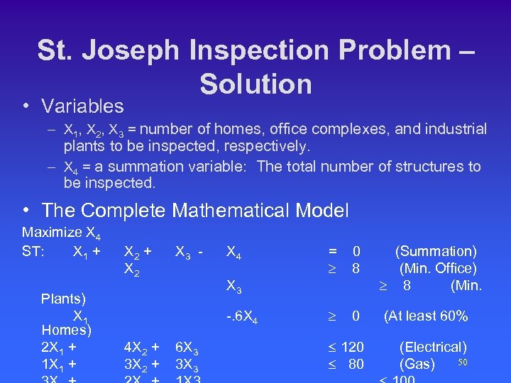 St. Joseph Inspection Problem – Solution • Variables – X 1, X 2, X 3 = number of homes, office complexes, and industrial plants to be inspected, respectively. – X 4 = a summation variable: The total number of structures to be inspected. • The Complete Mathematical Model Maximize X 4 ST: X 1 + Plants) X 1 Homes) 2 X 1 + 1 X 1 + X 2 X 3 - X 4 0 8 (Summation) (Min. Office) ³ 8 (Min. ³ 0 (At least 60% £ 120 £ 80 (Electrical) 50 (Gas) X 3 -. 6 X 4 4 X 2 + 3 X 2 + = ³ 6 X 3 3 X 3
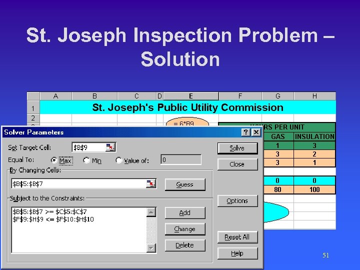 St. Joseph Inspection Problem – Solution 51
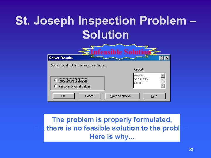 St. Joseph Inspection Problem – Solution Infeasible Solution The problem is properly formulated, but there is no feasible solution to the problem. Here is why. . . 52
 St. Joseph Inspection Problem spreadsheet Even when the smallest number allowed of offices and plants are inspected, the number of houses that can be inspected with the given resources is too small. Here is the reasoning. 53
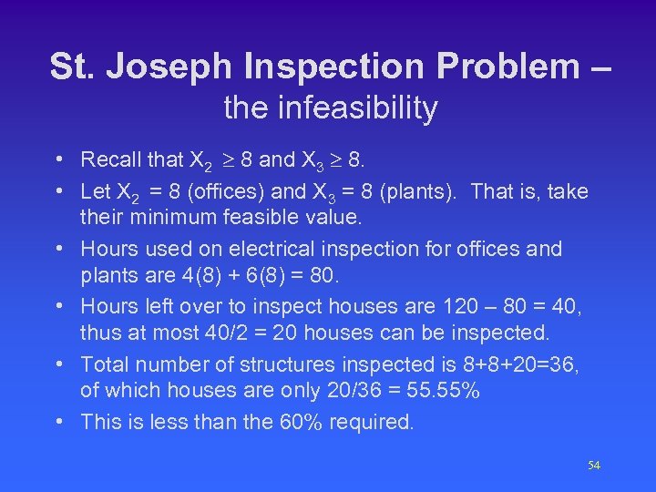 St. Joseph Inspection Problem – the infeasibility • Recall that X 2 ³ 8 and X 3 ³ 8. • Let X 2 = 8 (offices) and X 3 = 8 (plants). That is, take their minimum feasible value. • Hours used on electrical inspection for offices and plants are 4(8) + 6(8) = 80. • Hours left over to inspect houses are 120 – 80 = 40, thus at most 40/2 = 20 houses can be inspected. • Total number of structures inspected is 8+8+20=36, of which houses are only 20/36 = 55. 55% • This is less than the 60% required. 54
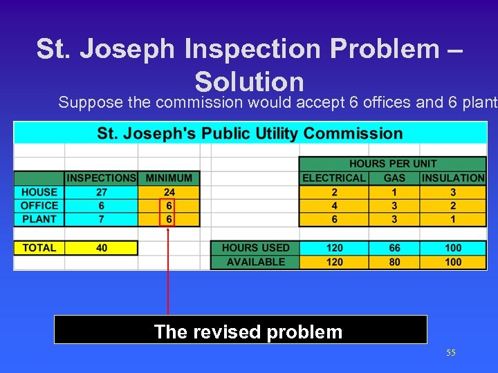 St. Joseph Inspection Problem – Solution Suppose the commission would accept 6 offices and 6 plants The revised problem 55
 3. 4. 4 Purchasing Modeling • These models can consider: – – – Demand Budget Cash flow Advertising Inventory restrictions. • In solving purchasing problems, we attempt to balance customer satisfaction with resource utilization by the business enterprise. 56
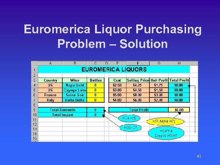
 Euromerica Liquor Purchasing Problem • Euromerica Liquors purchases and distributes a number of wines to retailers. • There are four different wines to be ordered. • Requirements – Order at least 800 of each type. – Order at least twice as many domestic bottles as imported bottles. 57
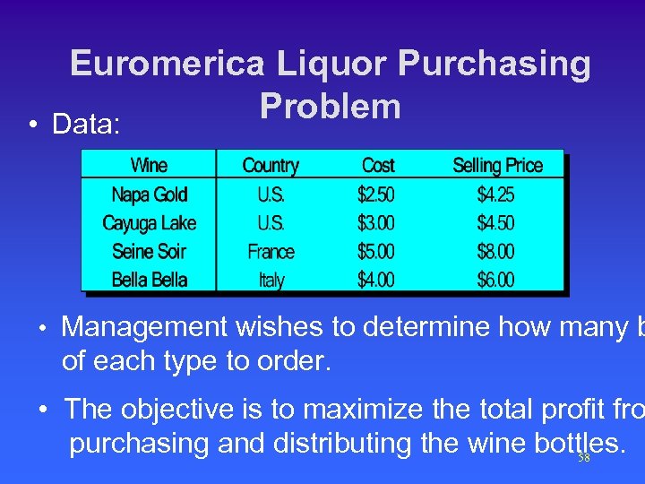 Euromerica Liquor Purchasing Problem • Data: • Management wishes to determine how many b of each type to order. • The objective is to maximize the total profit fro purchasing and distributing the wine bottles. 58
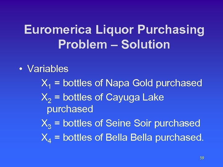 Euromerica Liquor Purchasing Problem – Solution • Variables X 1 = bottles of Napa Gold purchased X 2 = bottles of Cayuga Lake purchased X 3 = bottles of Seine Soir purchased X 4 = bottles of Bella purchased. 59
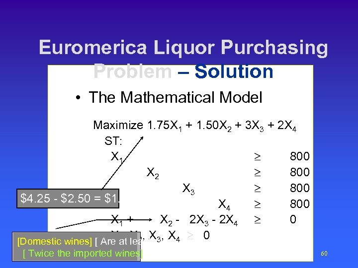 Euromerica Liquor Purchasing Problem – Solution • The Mathematical Model Maximize 1. 75 X 1 + 1. 50 X 2 + 3 X 3 + 2 X 4 ST: X 1 ³ 800 X 2 ³ 800 X 3 ³ 800 $4. 25 - $2. 50 = $1. 75 X 4 ³ 800 X 1 + X 2 - 2 X 3 - 2 X 4 ³ 0 X 1, X 2, X ³ 0 [Domestic wines] [ Are at least] 3 4 [ Twice the imported wines] 60
 Euromerica Liquor Purchasing Problem – Solution 61
 Euromerica Liquor Purchasing Problem – Solution An Unbounded solution 62
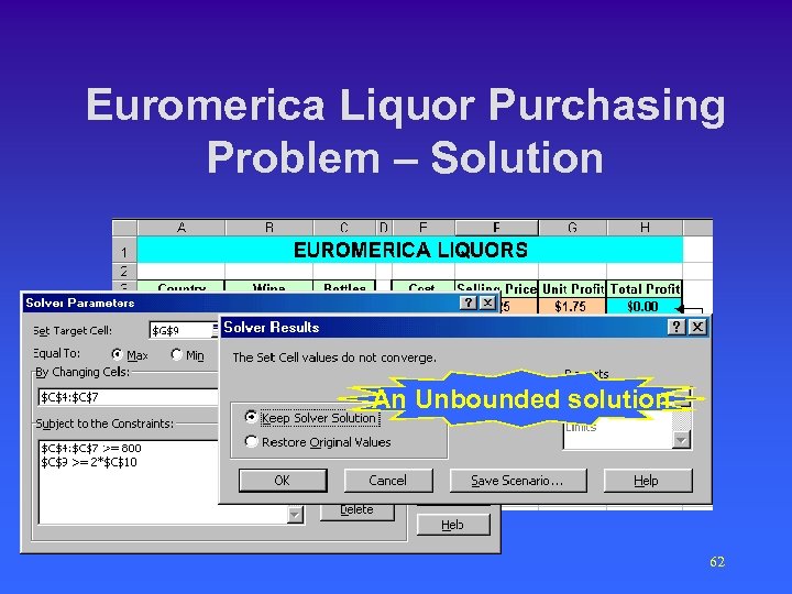
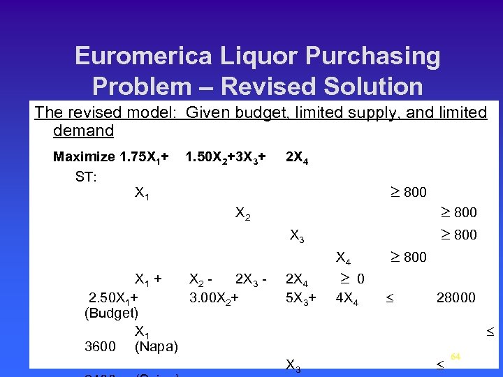
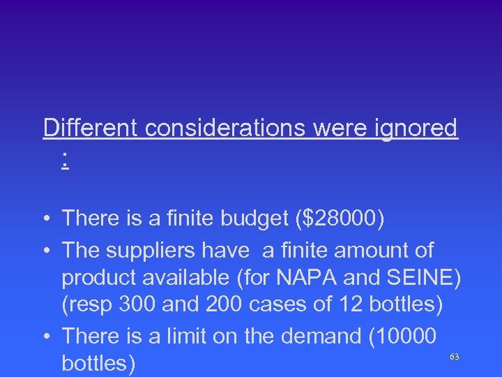 Different considerations were ignored : • There is a finite budget ($28000) • The suppliers have a finite amount of product available (for NAPA and SEINE) (resp 300 and 200 cases of 12 bottles) • There is a limit on the demand (10000 63 bottles)
 Euromerica Liquor Purchasing Problem – Revised Solution The revised model: Given budget, limited supply, and limited demand Maximize 1. 75 X 1+ ST: X 1 1. 50 X 2+3 X 3+ 2 X 4 ³ 800 X 2 X 3 X 4 X 1 + X 2 2 X 3 2. 50 X 1+ 3. 00 X 2+ (Budget) X 1 3600 (Napa) 2 X 4 5 X 3+ ³ 800 4 X 4 £ ³ 0 28000 £ X 3 £ 64
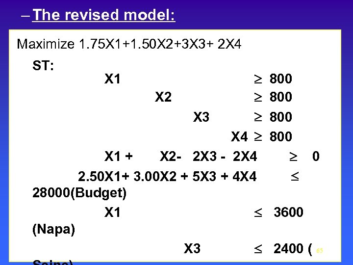 – The revised model: Maximize 1. 75 X 1+1. 50 X 2+3 X 3+ 2 X 4 ST: X 2 X 3 X 4 X 1 + X 2 - 2 X 3 - 2 X 4 2. 50 X 1+ 3. 00 X 2 + 5 X 3 + 4 X 4 28000(Budget) X 1 (Napa) X 3 X 1 800 800 0 3600 2400 ( 65
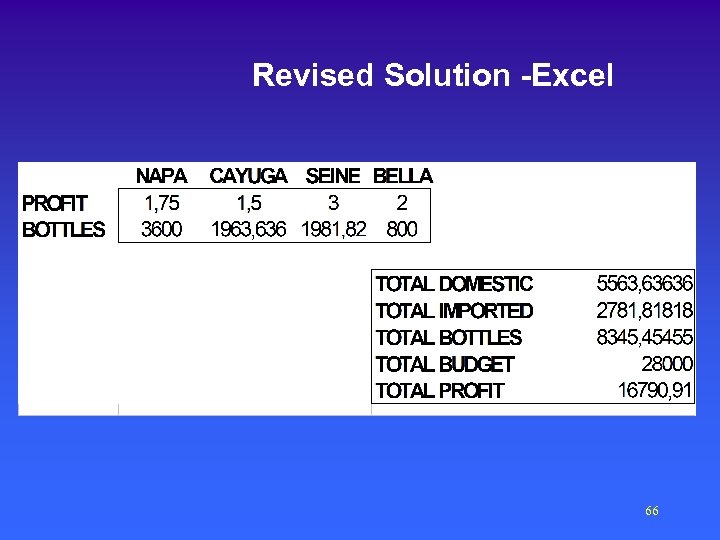 Revised Solution -Excel 66
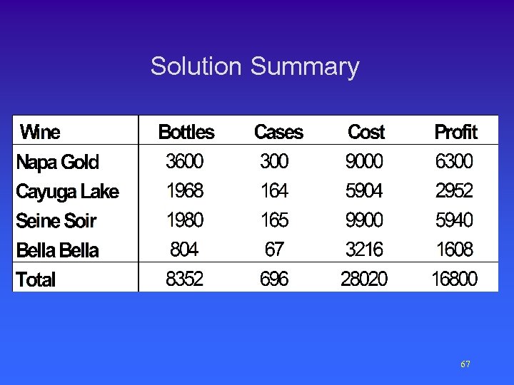 Solution Summary 67
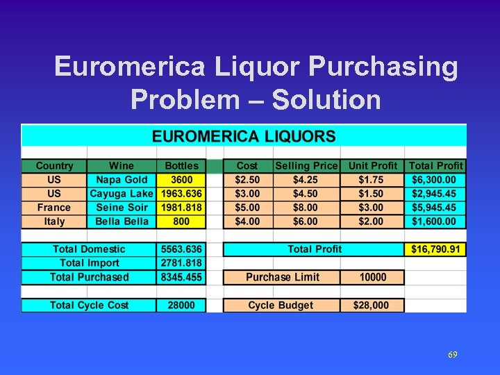 Euromerica Liquor Purchasing Problem – Solution 69
 3. 4. 5 Blending Models • Blending models were successfully implemented first by the oil industry. • Blending problems have the following characteristics: – Each of several products have certain specifications that must be met. – The products can be produced by blending various components, each with different properties of its own. – The problem is to find the least costly (most profitable) blends that meet the requirements and 70 specifications of all the products.
 United Oil Company • United Oil blends two input streams of crude oil – Alkylate – Catalytic Cracked. • The outputs of the blending process are – Regular gasoline. – Mid-Grade gasoline. – Premium gasoline. 71
 United Oil Company • Restrictions – Weekly supply of Crude oil is limited. – Contracted weekly demand for commercial gasoline has to be met. – To classify gasoline as Regular, Mid-Grade, or Premium, certain levels (specifications) of octane and vapor pressure must be met. • Profit per barrel of each type of commercial 72 gasoline depends on the blend it was made of.
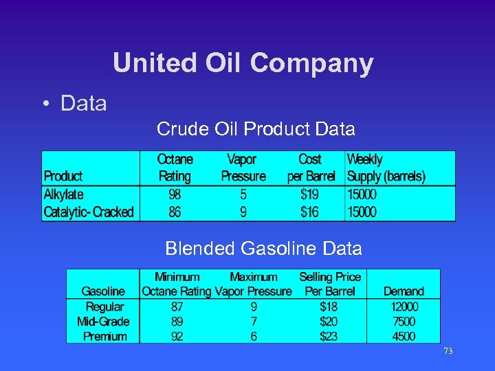 United Oil Company • Data Crude Oil Product Data Blended Gasoline Data 73
 United Oil Company • Problem Summary – Determine how many barrels of catalytic cracked to blend into regular, mid – grade, and premium each week. – Maximize total weekly profit. – Remain within raw gas availability. – Meet contract requirements. – Produce gasoline blends that meet the octane and vapor pressure requirements. 74
 United Oil Company – Solution • Decision Variables X 1, X 2, X 3 = number of barrels of Alkylate blended each week into Regular, Mid-Grade, and Premium gas respectively. Y 1, Y 2, Y 3 = number of barrels of Catalytic Cracked blended each week into Regular Mid-Grade, and Premium respectively. R, M, P = barrels of Regular, Mid-Grade, Premium respectively, produced weekly (summation variables). 75
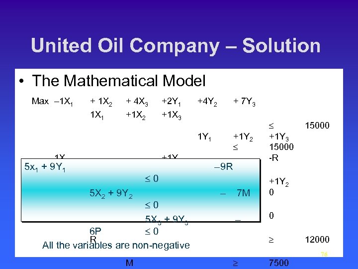 United Oil Company – Solution • The Mathematical Model Max – 1 X 1 + 1 X 2 + 4 X 3 +2 Y 1 1 X 1 +1 X 2 +4 Y 2 + 7 Y 3 +1 X 3 1 Y 1 1 X 1 5 x 1 + 9 Y 1 +1 Y 1 = Click for more 1 X 2 £ 0 constraints -M 5 X 2 + 9 Y 2 1 X 1 £ 0 0 5 X 3 + 9 Y 3 -P 6 P £ 0 R All the variables are non-negative M +1 Y 2 £ – 9 R – =7 M +1 Y 1 = – £ +1 Y 3 15000 -R +1 Y 2 0 0 ³ ³ 15000 12000 76 7500
 77
77
 78
78
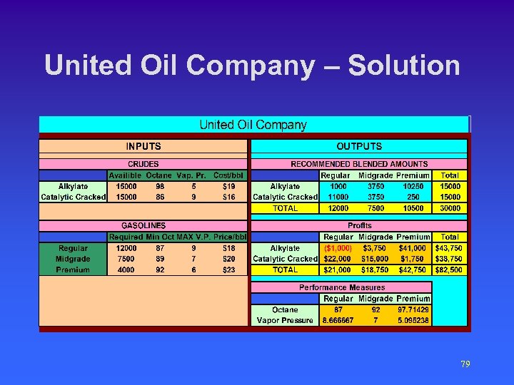 United Oil Company – Solution 79
 Appendix 3. 2 (CD): Cash Flow Models • These models cover a planning horizon of several periods. • Linking constraints secure the proper transfer of quantities from one period to the next one. The form of these constraints is: Amount this period = Amount last period + Inflow for the period – Outflow for the period • These models are useful for accounting analysis. 80
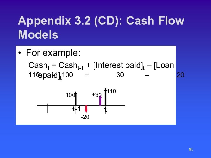 Appendix 3. 2 (CD): Cash Flow Models • For example: Casht = Casht-1 + [Interest paid]t – [Loan 110 = 30 – 20 repaid]t 100 +30 t-1 110 t -20 81
 The Powers Group Cash Flow Problem • Data – There are $9 million available for short-term investments over a period of five months (it is now January 1). – There are three possible investments. – Interest earned on each investment is: • 0. 7% over two months for two month term account. • 1. 5% over three months for three months construction loan. • 0. 2% per one-month period for passbook saving account. – Funds invested in term account are not liquid before the term ends. 82
 The Powers Group Cash Flow Problem • Objective function – Maximize the book value at the end of May. • Constraints – No more than $4 million should be invested in any one of the three short term investments. – Total investment each month in the liquid passbook account should be at least $2 million. – Cash available at the end of each month should be at least $3. 5 million. – Cash available at the end of May should be at 83 least $5 million.
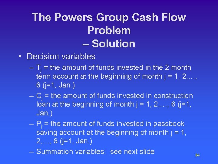 The Powers Group Cash Flow Problem – Solution • Decision variables – Tj = the amount of funds invested in the 2 month term account at the beginning of month j = 1, 2, …, 6 (j=1, Jan. ) – Cj = the amount of funds invested in construction loan at the beginning of month j = 1, 2, …, 6 (j=1, Jan. ) – Pj = the amount of funds invested in passbook saving account at the beginning of month j = 1, 2, …, 6 (j=1, Jan. ) – Summation variables: see next slide 84
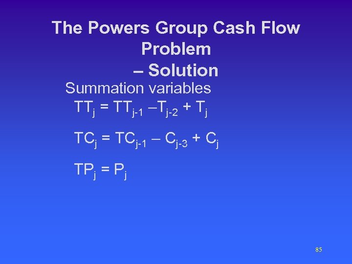 The Powers Group Cash Flow Problem – Solution Summation variables TTj = TTj-1 –Tj-2 + Tj TCj = TCj-1 – Cj-3 + Cj TPj = Pj 85
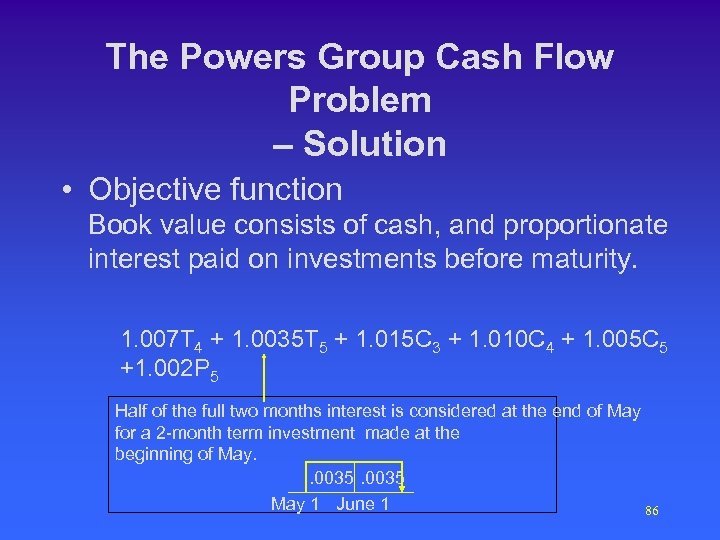 The Powers Group Cash Flow Problem – Solution • Objective function Book value consists of cash, and proportionate interest paid on investments before maturity. 1. 007 T 4 + 1. 0035 T 5 + 1. 015 C 3 + 1. 010 C 4 + 1. 005 C 5 +1. 002 P 5 Half of the full two months interest is considered at the end of May for a 2 -month term investment made at the beginning of May. . 0035 May 1 June 1 86
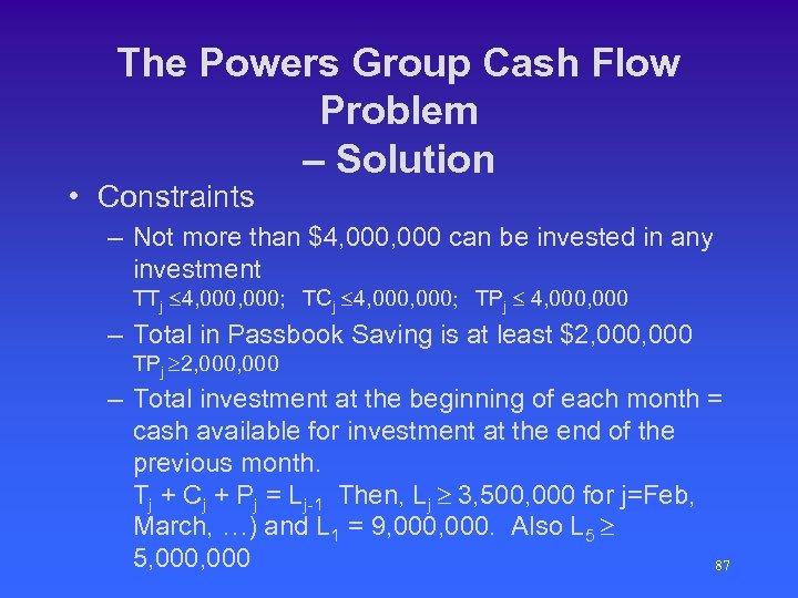 The Powers Group Cash Flow Problem – Solution • Constraints – Not more than $4, 000 can be invested in any investment TTj £ 4, 000; TCj £ 4, 000; TPj £ 4, 000 – Total in Passbook Saving is at least $2, 000 TPj ³ 2, 000 – Total investment at the beginning of each month = cash available for investment at the end of the previous month. Tj + Cj + Pj = Lj-1 Then, Lj ³ 3, 500, 000 for j=Feb, March, …) and L 1 = 9, 000. Also L 5 ³ 5, 000 87
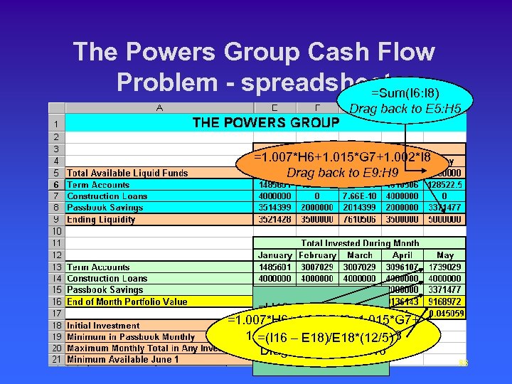 The Powers Group Cash Flow Problem - spreadsheet =Sum(I 6: I 8) Drag back to E 5: H 5 =1. 007*H 6+1. 015*G 7+1. 002*I 8 Drag back to E 9: H 9 =H 13+I 6 -G 6 =1. 007*H 6+1. 0035*I 6+1. 015*G 7+ =H 14+I&7 -G 7 1. 01*H 7+1. 005*I 7+1. 002*I 8 =(I 16 – E 18)/E 18*(12/5) =I 8 Drag back to E 16: H 16 Drag back to column E: H 88
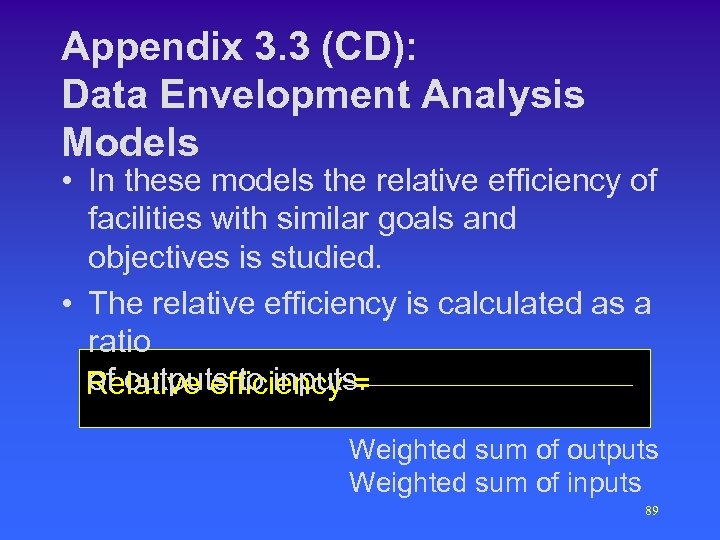 Appendix 3. 3 (CD): Data Envelopment Analysis Models • In these models the relative efficiency of facilities with similar goals and objectives is studied. • The relative efficiency is calculated as a ratio of outputs to inputs. Relative efficiency = Weighted sum of outputs Weighted sum of inputs 89
 Sir Loin Restaurants - DEA • KATTLECORP Inc. owns and operates four restaurants located in different states. • The restaurants are of different size, personnel, and traffic density. • KATTLECORP wishes to determine which restaurant operates efficiently. 90
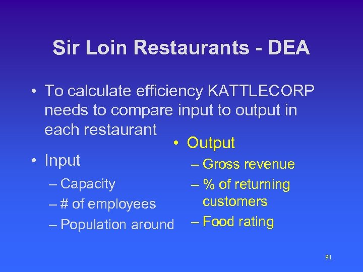 Sir Loin Restaurants - DEA • To calculate efficiency KATTLECORP needs to compare input to output in each restaurant • Output • Input – Gross revenue – Capacity – # of employees – Population around – % of returning customers – Food rating 91
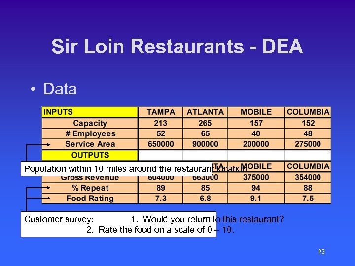 Sir Loin Restaurants - DEA • Data Population within 10 miles around the restaurant location Customer survey: 1. Would you return to this restaurant? 2. Rate the food on a scale of 0 – 10. 92
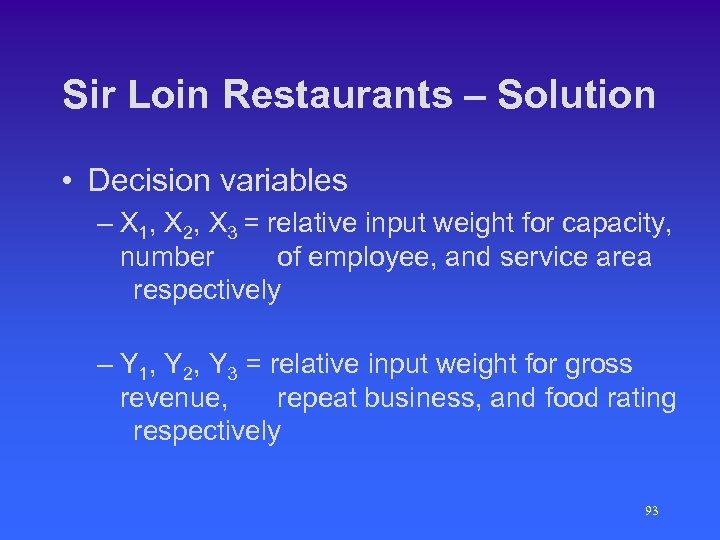 Sir Loin Restaurants – Solution • Decision variables – X 1, X 2, X 3 = relative input weight for capacity, number of employee, and service area respectively – Y 1, Y 2, Y 3 = relative input weight for gross revenue, repeat business, and food rating respectively 93
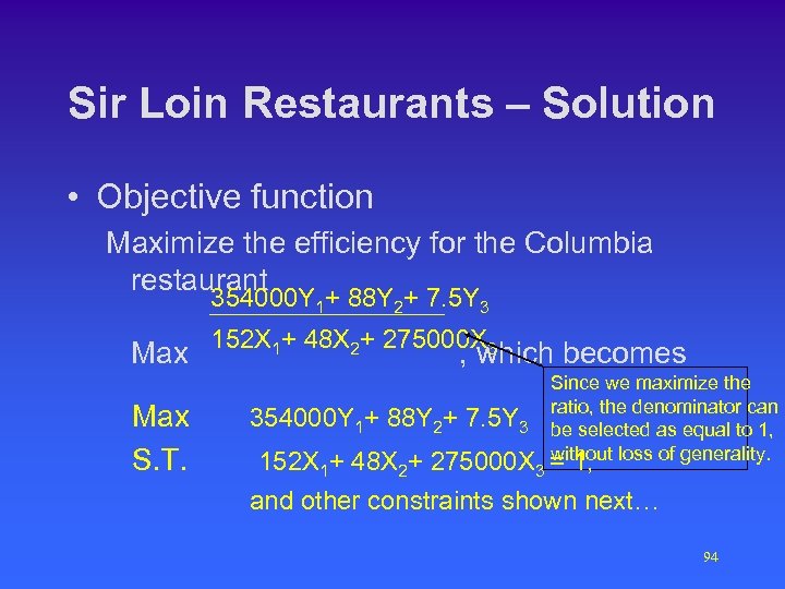 Sir Loin Restaurants – Solution • Objective function Maximize the efficiency for the Columbia restaurant 354000 Y 1+ 88 Y 2+ 7. 5 Y 3 Max S. T. 152 X 1+ 48 X 2+ 275000 X 3 , which becomes 354000 Y 1+ 88 Y 2+ 7. 5 Y 3 Since we maximize the ratio, the denominator can be selected as equal to 1, without loss of generality. 152 X 1+ 48 X 2+ 275000 X 3 = 1, and other constraints shown next… 94
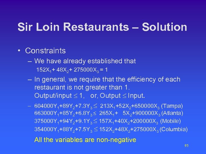 Sir Loin Restaurants – Solution • Constraints – We have already established that 152 X 1+ 48 X 2+ 275000 X 3 = 1 – In general, we require that the efficiency of each restaurant is not greater than 1. Output/input £ 1, or, Output £ Input. – 604000 Y 1+89 Y 2+7. 3 Y 3 £ 213 X 1+52 X 2+650000 X 3 (Tampa) 663000 Y 1+85 Y 2+6. 8 Y 3 £ 265 X 1+ 5 X 2+900000 X 3 (Atlanta) 375000 Y 1+94 Y 2+9. 1 Y 3 £ 157 X 1+40 X 2+200000 X 3 (Mobile) 354000 Y 1+88 Y 2+7. 5 Y 3 £ 152 X 2+48 X 2+275000 X 3 (Columbia) All the variables are non-negative 95
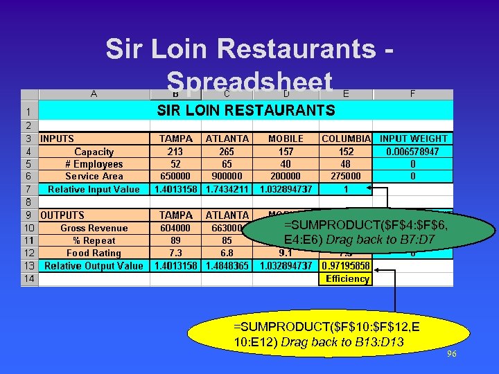 Sir Loin Restaurants Spreadsheet =SUMPRODUCT($F$4: $F$6, E 4: E 6) Drag back to B 7: D 7 =SUMPRODUCT($F$10: $F$12, E 10: E 12) Drag back to B 13: D 13 96


