Chapter 27 Inference for Simple Linear Regression 1

Chapter 27 Inference for Simple Linear Regression 1. review of least squares procedure 2. inference for least squares lines 1

Introduction • We will examine the relationship between quantitative variables x and y via a mathematical equation. • The motivation for using the technique: – Forecast the value of a resposne variable (y) from the value of explanatory variables (x 1, x 2, …xk. ). – Analyze the specific relationship between the explanatory variable and the dependent 2 variable.

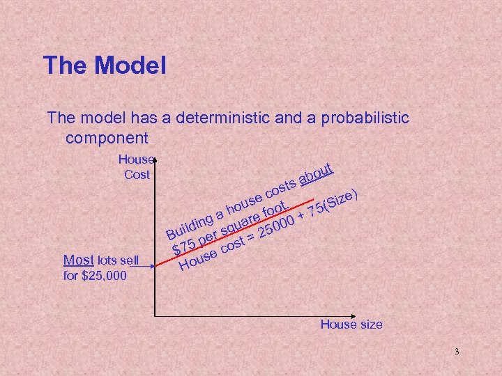The Model The model has a deterministic and a probabilistic component House Cost Most lots sell for $25, 000 out ab sts o e c t. ize) s (S ou a h re foo 0 + 75 ing qua 500 ld Bui per s t = 2 s $75 se co House size 3

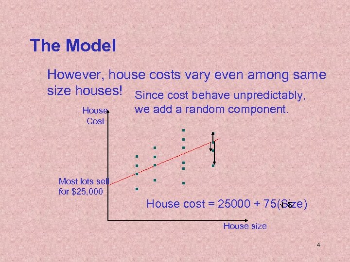The Model However, house costs vary even among same size houses! Since cost behave unpredictably, House Cost Most lots sell for $25, 000 we add a random component. +e House cost = 25000 + 75(Size) House size 4

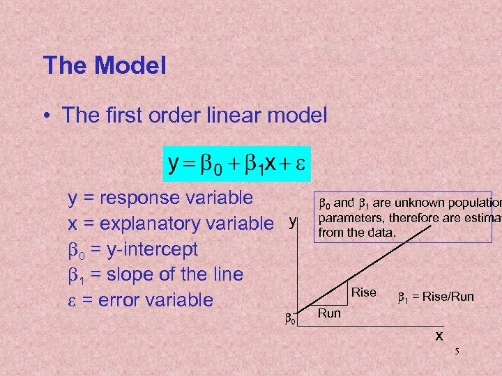The Model • The first order linear model y = response variable x = explanatory variable y b 0 = y-intercept b 1 = slope of the line e = error variable b 0 and b 1 are unknown population parameters, therefore are estimat from the data. Rise b 1 = Rise/Run x 5

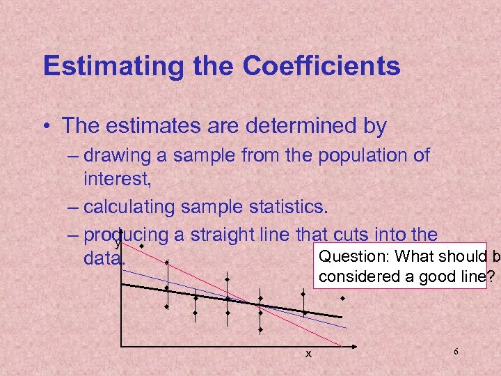Estimating the Coefficients • The estimates are determined by – drawing a sample from the population of interest, – calculating sample statistics. – producing a straight line that cuts into the y w Question: What should b data. w w w considered a good line? w w w x 6

The Least Squares (Regression) Line A good line is one that minimizes the sum of squared differences between the points and the line. 7

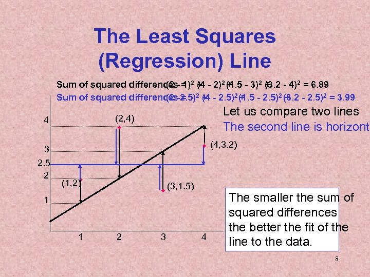The Least Squares (Regression) Line Sum of squared differences- = 2 + - 2)2 (1. 5 - 3)2 + - 4)2 = 6. 89 (2 1) (4 + (3. 2 Sum of squared differences-2. 5)2 + - 2. 5)2 (1. 5 - 2. 5)2 (3. 2 - 2. 5)2 = 3. 99 (2 = (4 + + 3 2. 5 2 Let us compare two lines The second line is horizonta (2, 4) w 4 w (4, 3. 2) w (1, 2) w (3, 1. 5) 1 1 2 3 4 The smaller the sum of squared differences the better the fit of the line to the data. 8

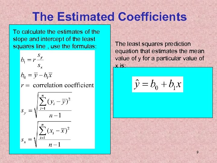The Estimated Coefficients To calculate the estimates of the slope and intercept of the least squares line , use the formulas: The least squares prediction equation that estimates the mean value of y for a particular value of x is: 9

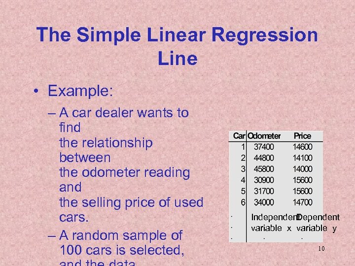The Simple Linear Regression Line • Example: – A car dealer wants to find the relationship between the odometer reading and the selling price of used cars. – A random sample of 100 cars is selected, Independent Dependent variable x variable y 10

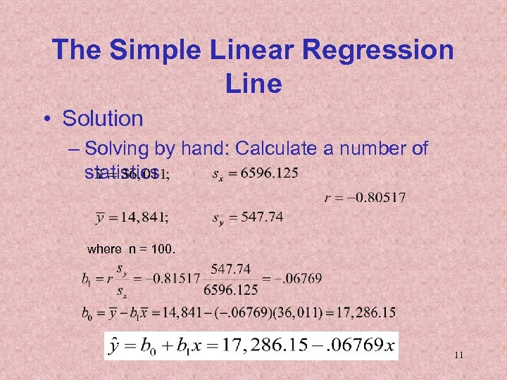The Simple Linear Regression Line • Solution – Solving by hand: Calculate a number of statistics where n = 100. 11

The Simple Linear Regression Line • Solution – continued – Using the computer 1. Scatterplot 2. Trend function 3. Data tab > Data Analysis > Regression 12

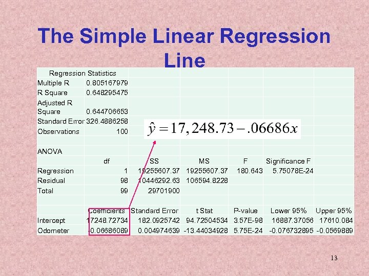The Simple Linear Regression Line Regression Statistics Multiple R 0. 805167979 R Square 0. 648295475 Adjusted R Square 0. 644706653 Standard Error 326. 4886258 Observations 100 ANOVA Regression Residual Total Intercept Odometer df 1 98 99 SS MS F Significance F 19255607. 37 180. 643 5. 75078 E-24 10446292. 63 106594. 8228 29701900 Coefficients Standard Error t Stat P-value Lower 95% Upper 95% 17248. 72734 182. 0925742 94. 72504534 3. 57 E-98 16887. 37056 17610. 084 -0. 06686089 0. 004974639 -13. 44034928 5. 75 E-24 -0. 076732895 -0. 0569889 13

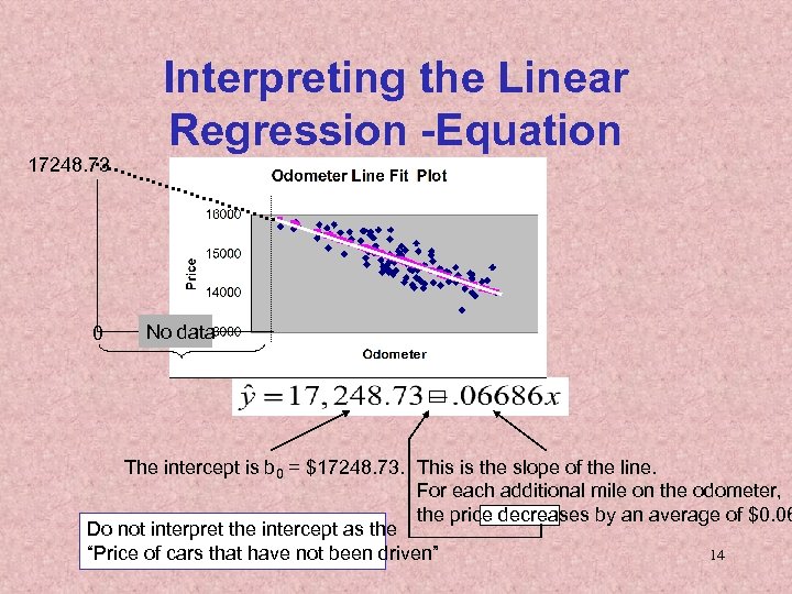17248. 73 0 Interpreting the Linear Regression -Equation No data The intercept is b 0 = $17248. 73. This is the slope of the line. For each additional mile on the odometer, the price decreases by an average of $0. 06 Do not interpret the intercept as the “Price of cars that have not been driven” 14

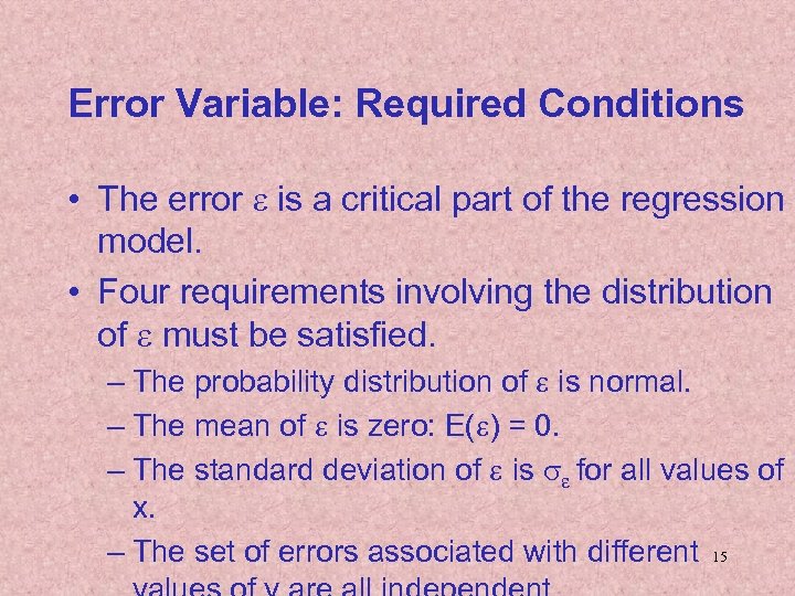Error Variable: Required Conditions • The error e is a critical part of the regression model. • Four requirements involving the distribution of e must be satisfied. – The probability distribution of e is normal. – The mean of e is zero: E(e) = 0. – The standard deviation of e is se for all values of x. – The set of errors associated with different 15

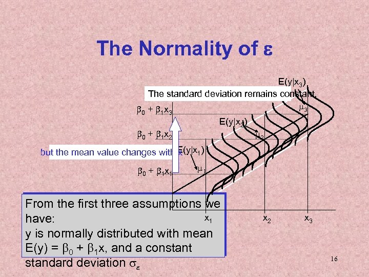The Normality of e E(y|x 3) The standard deviation remains constant, m 3 b 0 + b 1 x 3 E(y|x 2) b 0 + b 1 x 2 m 2 E(y|x 1) but the mean value changes with x b 0 + b 1 x 1 m 1 From the first three assumptions we x 1 have: y is normally distributed with mean E(y) = b 0 + b 1 x, and a constant standard deviation se x 2 x 3 16

Assessing the Model • The least squares method will produces a regression line whether or not there is a linear relationship between x and y. • Consequently, it is important to assess how well the linear model fits the data. • Several methods are used to assess the model. All are based on the sum of squares for errors, SSE. 17

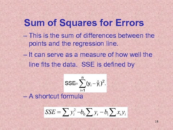Sum of Squares for Errors – This is the sum of differences between the points and the regression line. – It can serve as a measure of how well the line fits the data. SSE is defined by – A shortcut formula 18

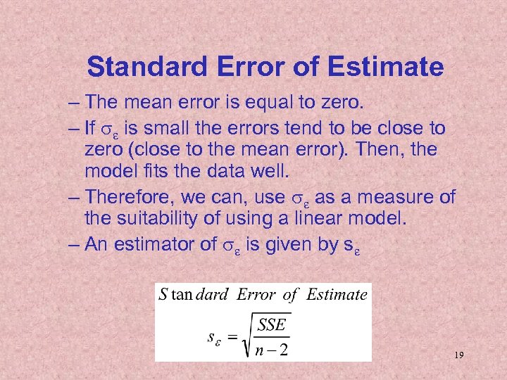Standard Error of Estimate – The mean error is equal to zero. – If se is small the errors tend to be close to zero (close to the mean error). Then, the model fits the data well. – Therefore, we can, use se as a measure of the suitability of using a linear model. – An estimator of se is given by se 19

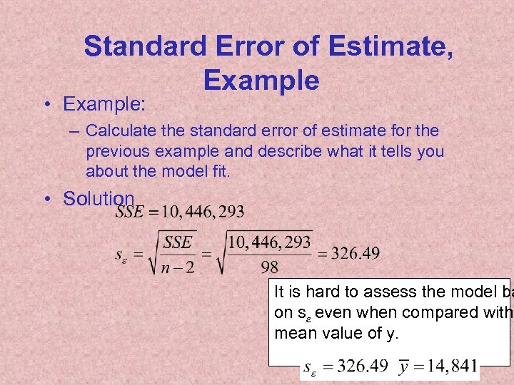Standard Error of Estimate, Example • Example: – Calculate the standard error of estimate for the previous example and describe what it tells you about the model fit. • Solution It is hard to assess the model ba on se even when compared with mean value of y. 20

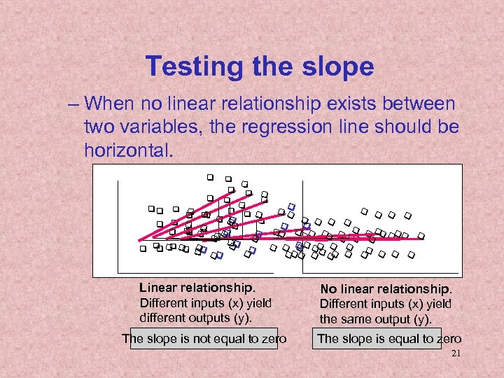Testing the slope – When no linear relationship exists between two variables, the regression line should be horizontal. q q qq q q q q q q q qq q q q qqq q q q q q q q qq q q q qqq q qq Linear relationship. Different inputs (x) yield different outputs (y). No linear relationship. Different inputs (x) yield the same output (y). The slope is not equal to zero The slope is equal to zero 21

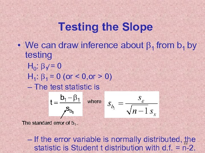Testing the Slope • We can draw inference about b 1 from b 1 by testing H 0: b 1 = 0 H 1: b 1 = 0 (or < 0, or > 0) – The test statistic is where The standard error of b 1. – If the error variable is normally distributed, the 22 statistic is Student t distribution with d. f. = n-2.

Testing the Slope, Example • Example – Test to determine whethere is enough evidence to infer that there is a linear relationship between the car auction price and the odometer reading for all three-year -old Tauruses in the previous example. Use a = 5%. 23

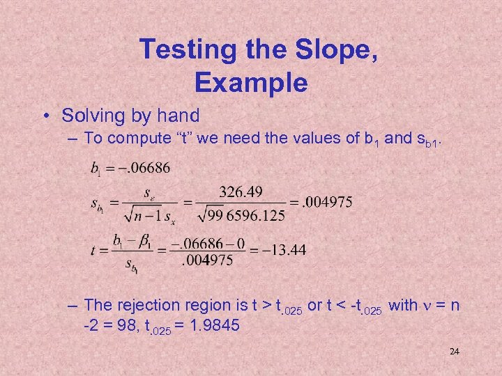Testing the Slope, Example • Solving by hand – To compute “t” we need the values of b 1 and sb 1. – The rejection region is t > t. 025 or t < -t. 025 with n = n -2 = 98, t. 025 = 1. 9845 24

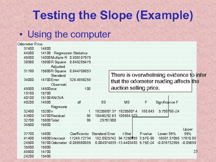Testing the Slope (Example) • Using the computer Odometer Price 37400 14600 44800 14100 Regression Statistics 45800 14000 Multiple R 0. 805167979 30900 15600 R Square 0. 648295475 Adjusted 31700 15600 R Square 0. 644706653 Standard 34000 14700 Error 326. 4886258 Observati 45900 14500 ons 100 19100 15700 40100 15100 ANOVA 40200 14800 df Regressio 32400 15200 n 1 43500 14700 Residual 98 32700 15600 Total 99 34500 15600 37700 41400 24500 35800 48600 24200 There is overwhelming evidence to infer that the odometer reading affects the auction selling price. SS MS F Significance F 19255607. 37 19255607. 4 180. 643 5. 75078 E-24 10446292. 63 106594. 823 29701900 Upper 14600 Coefficients Standard Error t Stat P-value Lower 95% 14600 Intercept 17248. 72734 182. 0925742 94. 7250453 3. 57 E-98 16887. 37056 17610. 08 15700 Odometer -0. 066860885 0. 004974639 -13. 4403493 5. 75 E-24 -0. 076732895 -0. 05699 15000 25 14700 15400

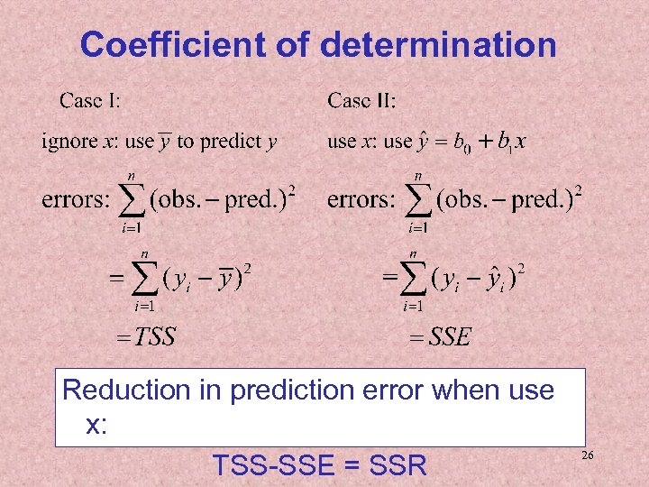Coefficient of determination Reduction in prediction error when use x: TSS-SSE = SSR 26

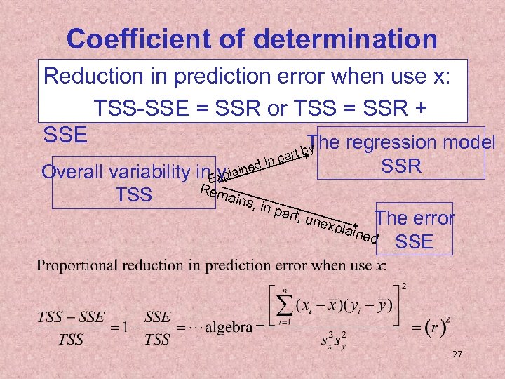Coefficient of determination Reduction in prediction error when use x: TSS-SSE = SSR or TSS = SSR + SSE The regression model y t b par d in Overall variability in yplaine Ex Rem ains TSS , in part , une SSR The error ined SSE xpla 27

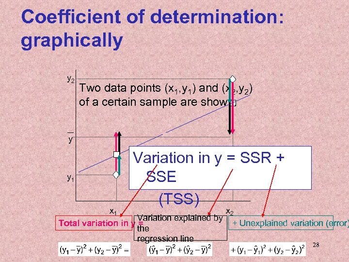Coefficient of determination: graphically y 2 Two data points (x 1, y 1) and (x 2, y 2) of a certain sample are shown. y y 1 Variation in y = SSR + SSE (TSS) x 1 x 2 Variation explained by + Unexplained variation (error) Total variation in y = the regression line 28

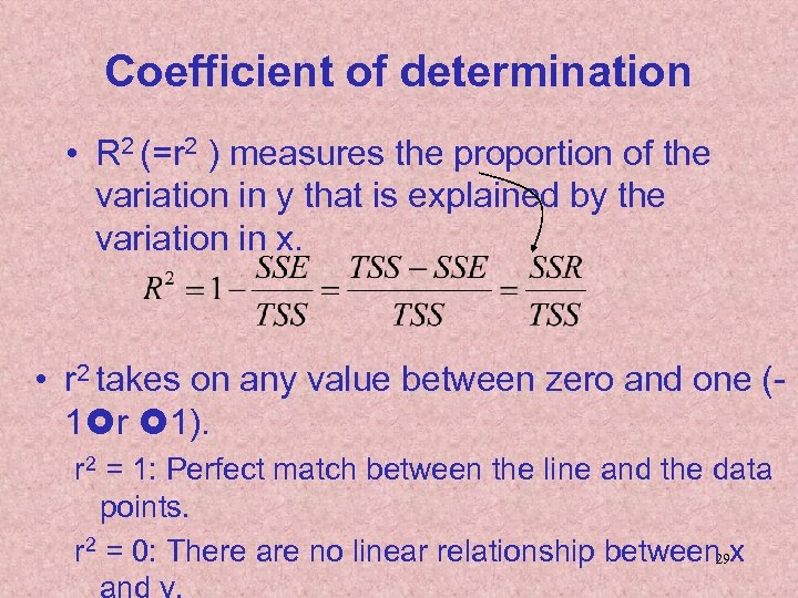Coefficient of determination • R 2 (=r 2 ) measures the proportion of the variation in y that is explained by the variation in x. • r 2 takes on any value between zero and one (1 r 1). r 2 = 1: Perfect match between the line and the data points. r 2 = 0: There are no linear relationship between x 29

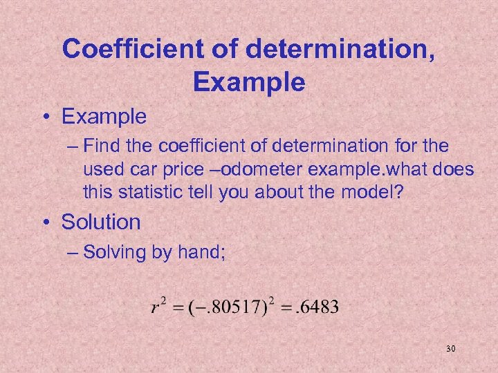Coefficient of determination, Example • Example – Find the coefficient of determination for the used car price –odometer example. what does this statistic tell you about the model? • Solution – Solving by hand; 30

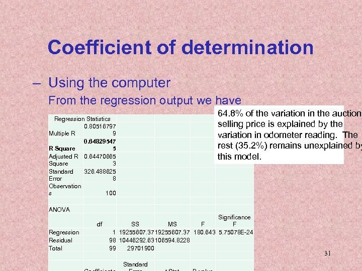Coefficient of determination – Using the computer From the regression output we have 64. 8% of the variation in the auction selling price is explained by the variation in odometer reading. The rest (35. 2%) remains unexplained by this model. Regression Statistics 0. 80516797 Multiple R 9 0. 64829547 R Square 5 Adjusted R 0. 64470665 Square 3 Standard 326. 488625 Error 8 Observation s 100 ANOVA Regression Residual Total df Significance SS MS F F 1 19255607. 37 180. 643 5. 75078 E-24 98 10446292. 63106594. 8228 99 29701900 Standard 31

Using the Regression Equation • Before using the regression model, we need to assess how well it fits the data. • If we are satisfied with how well the model fits the data, we can use it to predict the values of y. • To make a prediction we use – Point prediction, and – Interval prediction 32

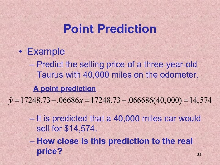Point Prediction • Example – Predict the selling price of a three-year-old Taurus with 40, 000 miles on the odometer. A point prediction – It is predicted that a 40, 000 miles car would sell for $14, 574. – How close is this prediction to the real price? 33

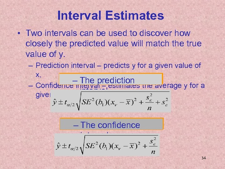Interval Estimates • Two intervals can be used to discover how closely the predicted value will match the true value of y. – Prediction interval – predicts y for a given value of x, – The prediction – Confidence interval – estimates the average y for a interval given x. – The confidence interval 34

Interval Estimates, Example • Example - continued – Provide an interval estimate for the bidding price on a Ford Taurus with 40, 000 miles on the odometer. – Two types of predictions are required: • A prediction for a specific car • An estimate for the average price per car 35

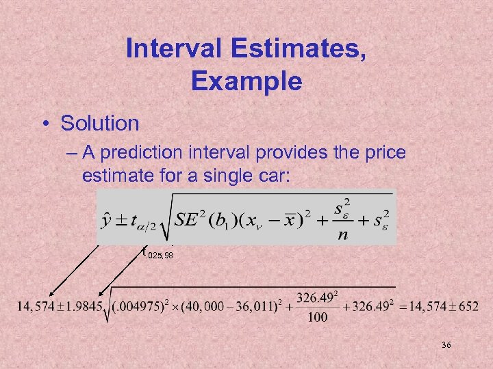Interval Estimates, Example • Solution – A prediction interval provides the price estimate for a single car: t. 025, 98 36

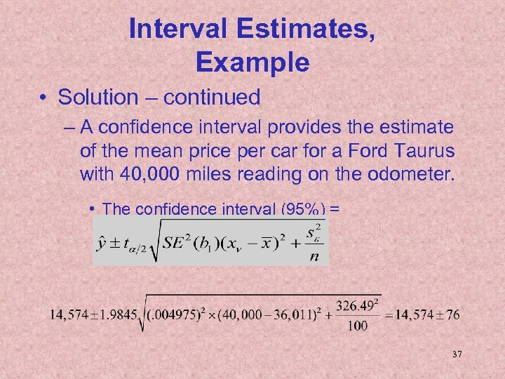Interval Estimates, Example • Solution – continued – A confidence interval provides the estimate of the mean price per car for a Ford Taurus with 40, 000 miles reading on the odometer. • The confidence interval (95%) = 37

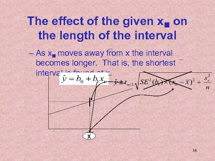The effect of the given x on the length of the interval – As x moves away from x the interval becomes longer. That is, the shortest interval is found at x. 38

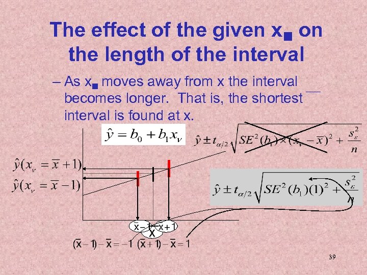The effect of the given x on the length of the interval – As x moves away from x the interval becomes longer. That is, the shortest interval is found at x. 39

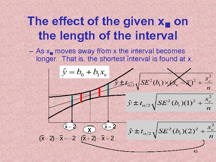The effect of the given x on the length of the interval – As x moves away from x the interval becomes longer. That is, the shortest interval is found at x. 40

Regression Diagnostics - I • The three conditions required for the validity of the regression analysis are: – the error variable is normally distributed. – the error variance is constant for all values of x. – The errors are independent of each other. • How can we diagnose violations of these conditions? 41

Residual Analysis • Examining the residuals (or standardized residuals), help detect violations of the required conditions. • Example – continued: – Nonnormality. • Use Excel to obtain the standardized residual histogram. • Examine the histogram and look for a bell shaped. diagram with a mean close to zero. 42

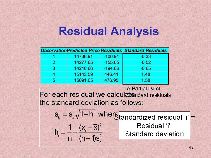Residual Analysis A Partial list of For each residual we calculate Standard residuals the standard deviation as follows: Standardized residual ‘i’ = Residual ‘i’ Standard deviation 43

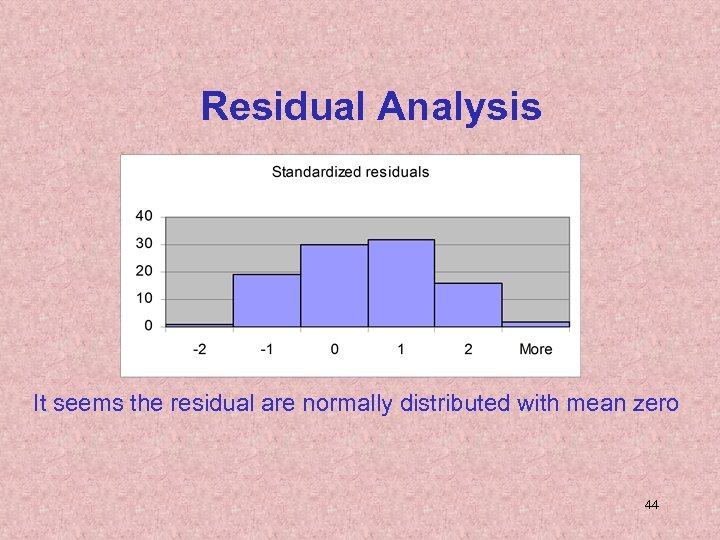Residual Analysis It seems the residual are normally distributed with mean zero 44

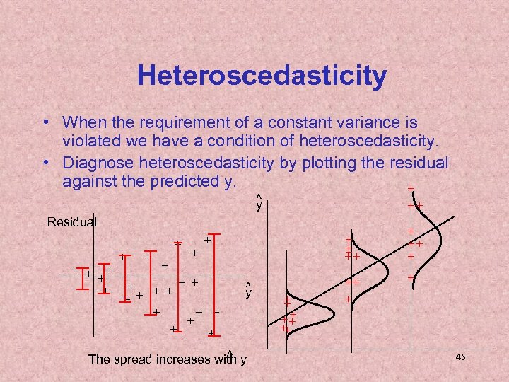Heteroscedasticity • When the requirement of a constant variance is violated we have a condition of heteroscedasticity. • Diagnose heteroscedasticity by plotting the residual against the predicted y. + ^ y ++ Residual + + + ++ + + + ^ y ^ The spread increases with y + ++ + + 45

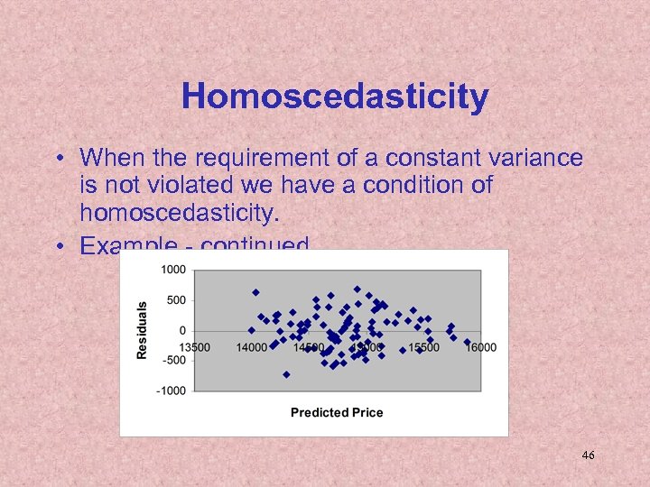Homoscedasticity • When the requirement of a constant variance is not violated we have a condition of homoscedasticity. • Example - continued 46

Non Independence of Error Variables – A time series is constituted if data were collected over time. – Examining the residuals over time, no pattern should be observed if the errors are independent. – When a pattern is detected, the errors are said to be autocorrelated. – Autocorrelation can be detected by graphing the residuals against time. 47

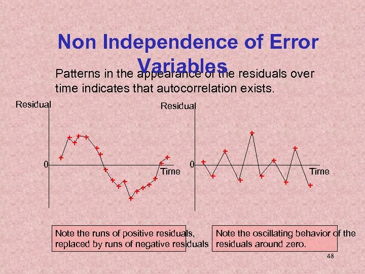Non Independence of Error Variables Patterns in the appearance of the residuals over time indicates that autocorrelation exists. Residual + ++ + 0 + + ++ + 0 + Time + + Note the runs of positive residuals, Note the oscillating behavior of the replaced by runs of negative residuals around zero. 48

Outliers • An outlier is an observation that is unusually small or large. • Several possibilities need to be investigated when an outlier is observed: – There was an error in recording the value. – The point does not belong in the sample. – The observation is valid. • Identify outliers from the scatter diagram. • It is customary to suspect an observation is an outlier if its |standard residual| > 2 49

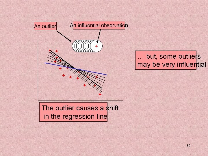An outlier An influential observation + + + + +++++ … but, some outliers may be very influential + + + + The outlier causes a shift in the regression line 50

Procedure for Regression Diagnostics • Develop a model that has a theoretical basis. • Gather data for the two variables in the model. • Draw the scatter diagram to determine whether a linear model appears to be appropriate. • Determine the regression equation. • Check the required conditions for the errors. • Check the existence of outliers and influential observations • Assess the model fit. • If the model fits the data, use the regression 51 equation.