Chapter 24 Perfect Competition Introduction A relatively

Chapter 24 Perfect Competition

Introduction A relatively new health care product offered for sale is the full-body CT scan. There are many firms offering this service, and yet they all charge nearly identical prices. Why would such a personal service not vary in price much between different providers? 2

Learning Objectives n Identify the characteristics of a perfectly competitive market structure n Discuss the process by which a perfectly competitive firm decides how much output to produce n Understand how the short-run supply curve for a perfectly competitive firm is determined 3

Learning Objectives n Explain how the equilibrium price is determined in a perfectly competitive market n Describe what factors induce firms to enter or exit a perfectly competitive industry n Distinguish among constant-, increasing-, and decreasing-cost industries based on the shape of the long-run industry supply curve 4

Chapter Outline n Characteristics of a Perfectly Competitive Market Structure n The Demand Curve of the Perfect Competitor n How Much Should the Perfect Competitor Produce? 5

Chapter Outline n Using Marginal Analysis to Determine the Profit. Maximizing Rate of Production n Short-Run Profits n The Short-Run Shutdown Price n The Perfect Competitor’s Short-Run Supply Curve 6

Chapter Outline n Competitive Price Determination n The Long-Run Industry Situation: Exit and Entry n Long-Run Equilibrium n Competitive Pricing: Marginal Cost Pricing 7

Did You Know That. . . n Clothing retailers commonly cite bad weather as the reason for poor profit performance? n The competitive nature of this market best explains why profits are kept to a modest level? 8

Characteristics of a Perfectly Competitive Market Structure n Perfect Competition – A market structure in which the decisions of individual buyers and sellers have no effect on market price 9

Characteristics of a Perfectly Competitive Market Structure n Perfectly Competitive Firm – A firm that is such a small part of the total industry that it cannot affect the price of the product or service that it sells 10

Characteristics of a Perfectly Competitive Market Structure n Price Taker – A competitive firm that must take the price of its product as given because the firm cannot influence its price 11

International Example: How Free Entry Can Shift Resources n In 1981, Chile began offering a program of school choice. n If parents decided to enroll their children in a private school, public funds would be made available to that school to cover all or part of tuition. 12

International Example: How Free Entry Can Shift Resources n Such a program reorders the incentives both for parents and schools. n Sinception of the program, more than 1, 200 new private schools have been formed. 13

Characteristics of a Perfectly Competitive Market Structure n Price taker: – A firm can sell as much as wants at the going market price. – There is no incentive to sell for a lower price. – Attempts to charge a higher price will result in no sales. 14

Characteristics of a Perfectly Competitive Market Structure n Characteristics of perfect competition – Large number of buyers and sellers – Homogenous products • When you buy a head of lettuce do you ask what farm it came from? – No barriers to entry or exit – Buyers and sellers have equal access to information 15

The Demand Curve of the Perfect Competitor n Question – If the perfectly competitive firm is a price taker, who or what sets the price? 16

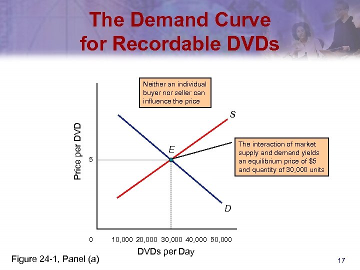The Demand Curve for Recordable DVDs Neither an individual buyer nor seller can influence the price Price per DVD S The interaction of market supply and demand yields an equilibrium price of $5 and quantity of 30, 000 units E 5 D 0 Figure 24 -1, Panel (a) 10, 000 20, 000 30, 000 40, 000 50, 000 DVDs per Day 17

The Demand Curve of the Perfect Competitor n The perfectly competitive firm: – Is a price taker (i. e. , must sell for $5) – Will sell all units for $5 – Will not be able to sell at a higher price – Will not choose to sell more units at a lower price 18

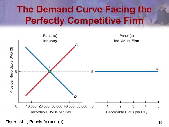The Demand Curve Facing the Perfectly Competitive Firm Figure 24 -1, Panels (a) and (b) 19

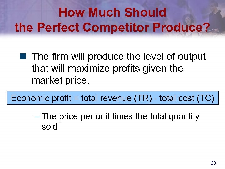How Much Should the Perfect Competitor Produce? n The firm will produce the level of output that will maximize profits given the market price. Economic profit = total revenue (TR) - total cost (TC) n Total Revenues – The price per unit times the total quantity sold 20

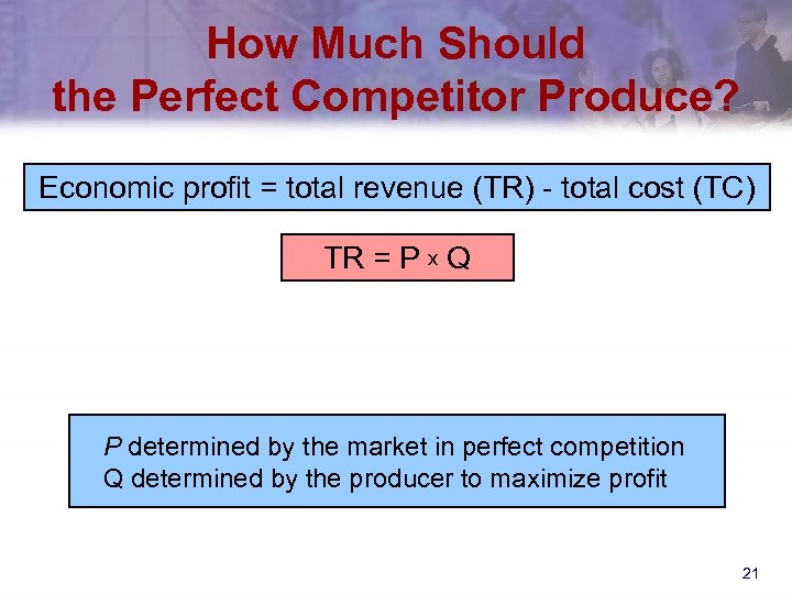How Much Should the Perfect Competitor Produce? Economic profit = total revenue (TR) - total cost (TC) TR = P x Q P determined by the market in perfect competition Q determined by the producer to maximize profit 21

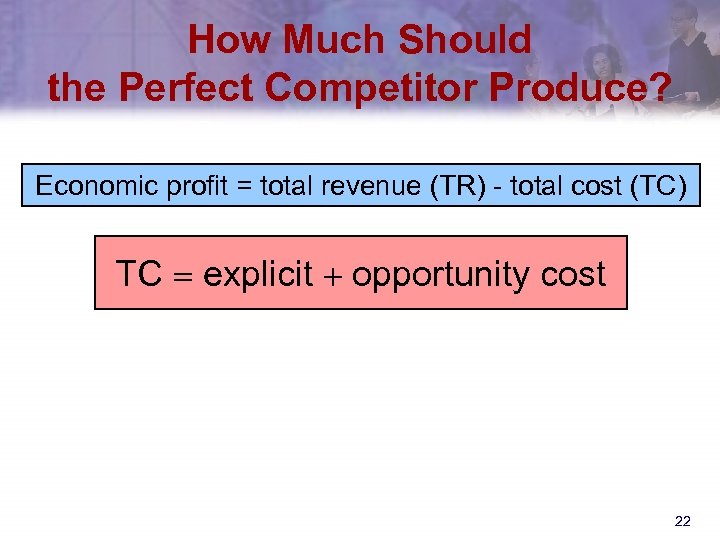How Much Should the Perfect Competitor Produce? Economic profit = total revenue (TR) - total cost (TC) TC explicit + opportunity cost 22

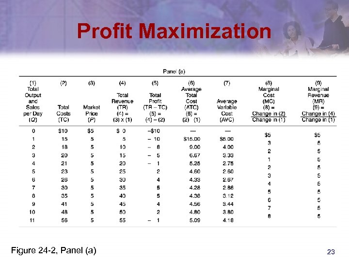Profit Maximization Figure 24 -2, Panel (a) 23

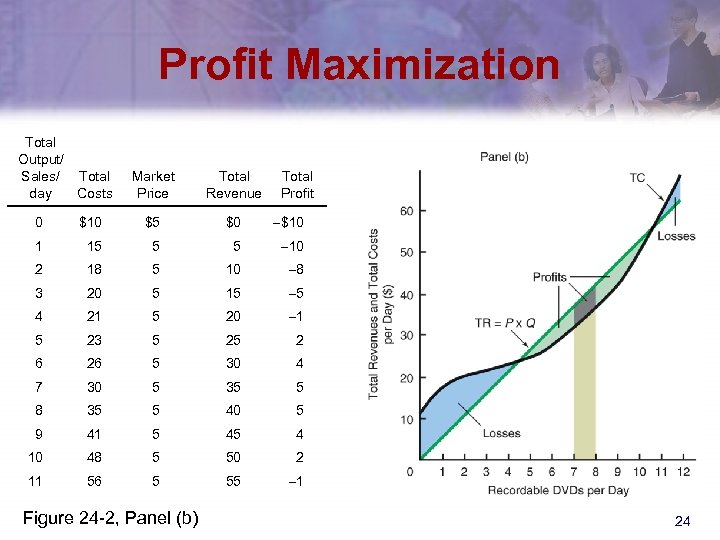Profit Maximization Total Output/ Sales/ Total day Costs Market Price Total Revenue Total Profit 0 $10 $5 $0 $10 1 15 5 5 10 2 18 5 10 8 3 20 5 15 5 4 21 5 20 1 5 23 5 25 2 6 26 5 30 4 7 30 5 35 5 8 35 5 40 5 9 41 5 45 4 10 48 5 50 2 11 56 5 55 1 Figure 24 -2, Panel (b) 24

How Much Should the Perfect Competitor Produce? n Profit-maximizing rate of production – The rate of production that maximizes total profits, or the difference between total revenues and total costs – Also, the rate of production at which marginal revenue equals marginal cost 25

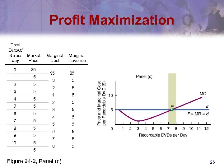Profit Maximization Total Output/ Sales/ Market day Price 0 $5 1 5 2 5 3 5 4 5 5 5 6 5 7 5 8 5 9 5 10 5 11 5 Marginal Cost Marginal Revenue $5 $5 3 5 2 5 1 5 2 5 3 5 4 5 5 5 6 5 7 5 8 5 Figure 24 -2, Panel (c) 26

Using Marginal Analysis to Determine the Profit-Maximizing Rate of Production n Marginal revenue is the change in total revenue divided by the change in output n Marginal cost is the change in total cost divided by the change in output 27

Using Marginal Analysis to Determine the Profit-Maximizing Rate of Production n Profit maximization – Economic profits = TR TC – Profit-maximizing output occurs when MC = MR – For a perfectly competitive firm, this is at the intersection of the firm’s demand schedule and its marginal cost curve 28

Short-Run Profits n To find out what our competitive individual DVD producer is making in terms of profits in the short run, we have to determine the excess of price above average total cost 29

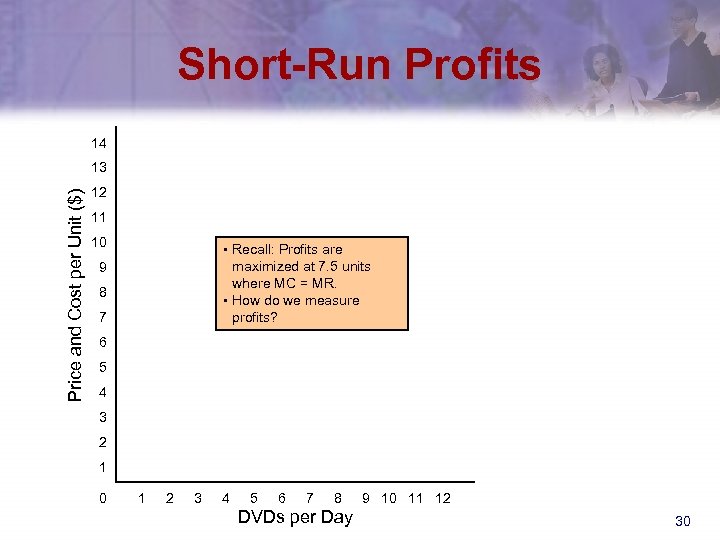Short-Run Profits 14 Price and Cost per Unit ($) 13 12 11 10 • Recall: Profits are maximized at 7. 5 units where MC = MR. • How do we measure profits? 9 8 7 6 5 4 3 2 1 0 1 2 3 4 5 6 7 8 DVDs per Day 9 10 11 12 30

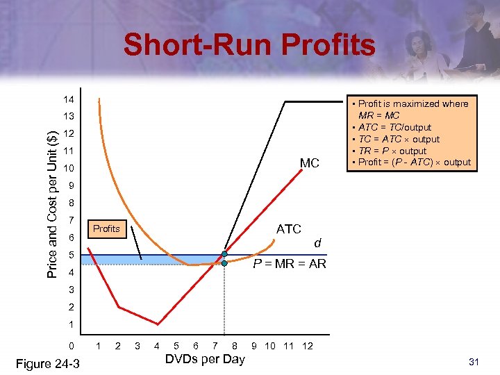Short-Run Profits 14 Price and Cost per Unit ($) 13 12 11 MC 10 • Profit is maximized where MR = MC • ATC = TC/output • TC = ATC output • TR = P output • Profit = (P - ATC) output 9 8 7 6 ATC Profits 5 d P = MR = AR 4 3 2 1 0 Figure 24 -3 1 2 3 4 5 6 7 8 DVDs per Day 9 10 11 12 31

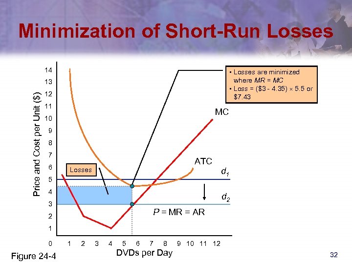Minimization of Short-Run Losses 14 • Losses are minimized where MR = MC • Loss = ($3 - 4. 35) 5. 5 or $7. 43 Price and Cost per Unit ($) 13 12 11 MC 10 9 8 7 6 ATC Losses 5 4 d 1 d 2 3 P = MR = AR 2 1 0 Figure 24 -4 1 2 3 4 5 6 7 8 DVDs per Day 9 10 11 12 32

Short-Run Profits n Short-run average profits or average losses are determined by comparing average total costs with price (average revenue) at the profit-maximizing rate of output. n In the short run, the perfectly competitive firm can make economic profits or economic losses. 33

The Short-Run Shutdown Price n What do you think? – Would you continue to produce if you were incurring a loss? • In the short run? • In the long run? 34

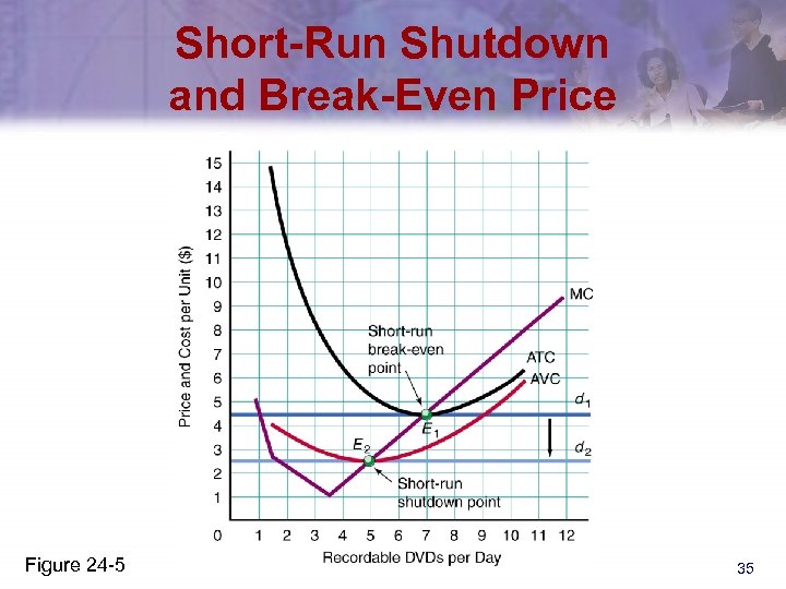Short-Run Shutdown and Break-Even Price Figure 24 -5 35

The Short-Run Shutdown Price n What do you think? – Would you continue to produce if you were incurring a loss? • In the short run? • In the long run? 36

The Short-Run Shutdown Price n As long as the price per unit sold exceeds the average variable cost per unit produced, the firm will be covering at least part of the opportunity cost of the investment in the business—that is, part of its fixed costs. 37

The Short-Run Shutdown Price n Short-Run Break-Even Price – The price at which a firm’s total revenues equal its costs – At the break-even price, the firm is just making a normal rate of return on its capital investment n Short-Run Shutdown Price – The price that just covers average variable costs – It occurs just below the intersection of the marginal cost curve and the average variable cost curve 38

The Meaning of Zero Economic Profits n Why produce if you are not making a profit? n Hint: – Distinguish between economic profits and accounting profits – When economic profits are zero, accounting profits are positive 39

The Perfect Competitor’s Short-Run Supply Curve n Question – What does the supply curve for the individual firm look like? n Answer – The firm’s supply curve is the marginal cost curve above the short-run shutdown point. – Thus, the competitive firm’s short-run supply curve is its marginal costs curve equal to and above the point of intersection with the average variable cost curve. 40

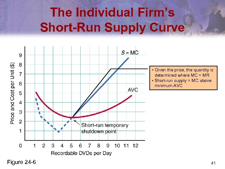The Individual Firm’s Short-Run Supply Curve • Given the price, the quantity is determined where MC = MR • Short-run supply = MC above minimum AVC Figure 24 -6 41

The Perfect Competitor’s Short-Run Supply Curve n The Industry Supply Curve – The locus of points showing the minimum prices at which given quantities will be forthcoming 42

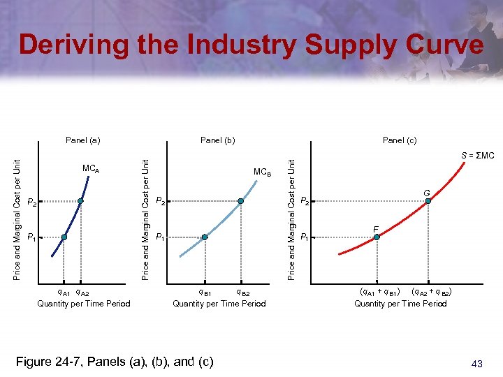Deriving the Industry Supply Curve P 2 P 1 q A 2 Quantity per Time Period Panel (c) MCB P 2 P 1 q B 2 Quantity per Time Period Figure 24 -7, Panels (a), (b), and (c) Price and Marginal Cost per Unit MCA Panel (b) Price and Marginal Cost per Unit Panel (a) S = ΣMC G P 2 P 1 F (q A 1 + q B 1) (q A 2 + q B 2) Quantity per Time Period 43

The Perfect Competitor’s Short-Run Supply Curve n Factors that influence the industry supply curve (determinants of supply) – Firm’s productivity – Factor costs – Taxes and subsidies – Number of firms 44

Competitive Price Determination n Question – How is the market, or “going, ” price established in a competitive market? n Answer – This price is established by the interaction of all the suppliers (firms) and all the demanders. 45

Competitive Price Determination n The competitive price is determined by the intersection of the market demand curve and the market supply curve – The market supply curve is equal to the horizontal summation of the supply curves of the individual firms 46

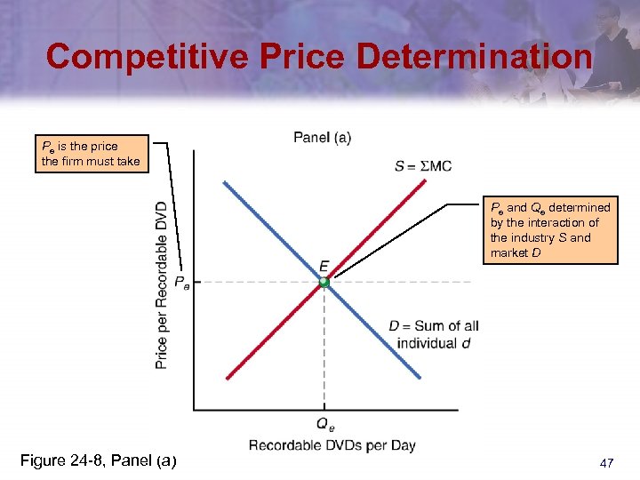Competitive Price Determination Pe is the price the firm must take Pe and Qe determined by the interaction of the industry S and market D Figure 24 -8, Panel (a) 47

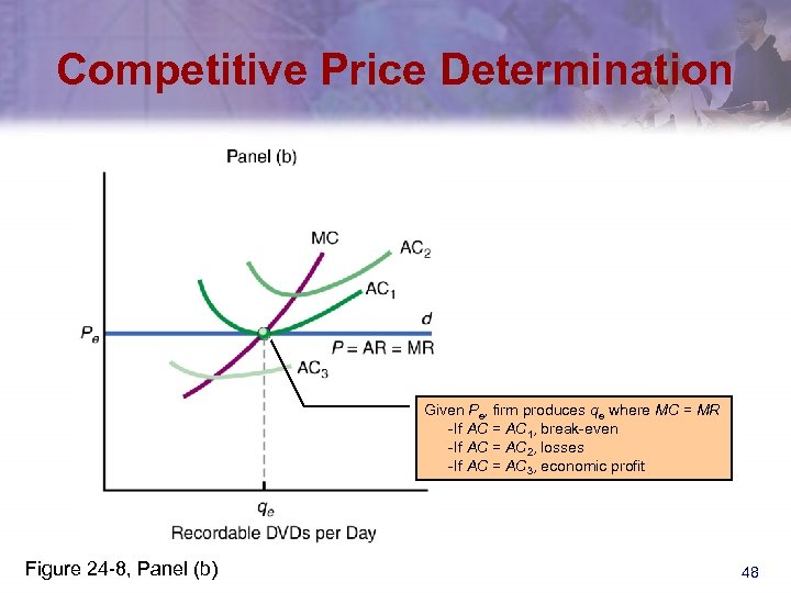Competitive Price Determination Given Pe, firm produces qe where MC = MR -If AC = AC 1, break-even -If AC = AC 2, losses -If AC = AC 3, economic profit Figure 24 -8, Panel (b) 48

The Long-Run Industry Situation: Exit and Entry n Profits and losses act as signals for resources to enter an industry or to leave an industry. 49

The Long-Run Industry Situation: Exit and Entry n Signals – Compact ways of conveying to economic decision makers information needed to make decisions – A true signal not only conveys information but also provides the incentive to react appropriately 50

The Long-Run Industry Situation: Exit and Entry n Summary – Economic profits • Signal resources to enter the market and the price falls to the break-even price – Economic losses • Signal resources to exit the market and the price increases to the break-even level 51

The Long-Run Industry Situation: Exit and Entry n Summary – At break-even • Resources will not enter or exit because the market is yielding a normal rate of return – In the long run, the perfectly competitive firm will make zero economic profits (a normal rate of return) 52

The Long-Run Industry Situation: Exit and Entry n Long-Run Industry Supply Curve – A market supply curve showing the relationship between price and quantities forthcoming after firms have been allowed time to enter or exit from an industry 53

The Long-Run Industry Situation: Exit and Entry n Constant-Cost Industry – An industry whose total output can be increased without an increase in long-run per-unit costs 54

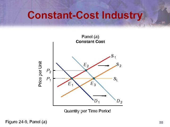Constant-Cost Industry Panel (a) Constant Cost Price per Unit S 1 S 2 E 2 P 1 E 3 D 1 SL D 2 Quantity per Time Period Figure 24 -9, Panel (a) 55

The Long-Run Industry Situation: Exit and Entry n Increasing-Cost Industry – An industry in which an increase in industry output is accompanied by an increase in long-run per unit costs 56

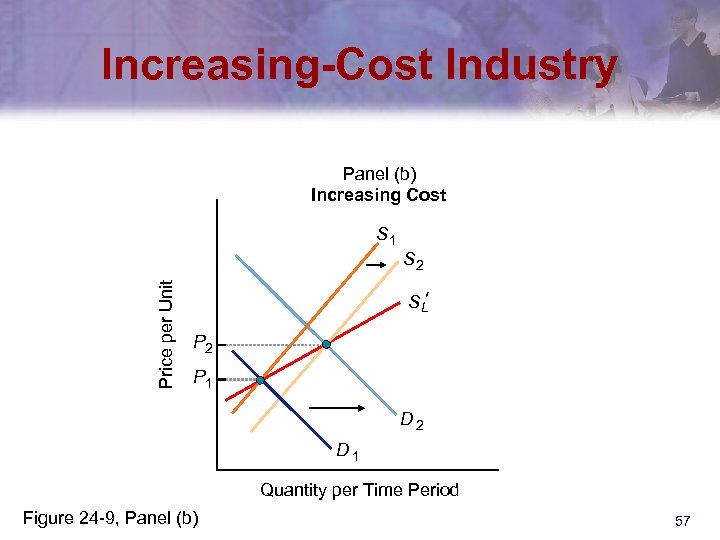Increasing-Cost Industry Panel (b) Increasing Cost S 1 Price per Unit S 2 ' SL P 2 P 1 D 2 D 1 Quantity per Time Period Figure 24 -9, Panel (b) 57

The Long-Run Industry Situation: Exit and Entry n Decreasing-Cost Industry – An industry in which an increase in industry output leads to a reduction in long -run per-unit costs 58

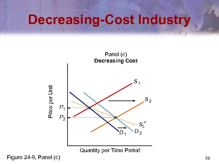Decreasing-Cost Industry Price per Unit Panel (c) Decreasing Cost S 1 S 2 P 1 P 2 '' SL D 1 D 2 Quantity per Time Period Figure 24 -9, Panel (c) 59

Example: The Market for Transistors n Since the late 1960’s, the annual production of transistors has expanded from 1 billion to 1 quintillion. n At the same time, the cost per unit has dropped from about $1 to a miniscule fraction of a penny. n Transistor production serves as a good illustration of a decreasing-cost industry. 60

Long-Run Equilibrium n Firms will adjust plant size until there is no further incentive to change. n In the long run, a competitive firm produces where price, marginal revenue, marginal cost, short-run minimum average cost, and long-run minimum average cost are equal. 61

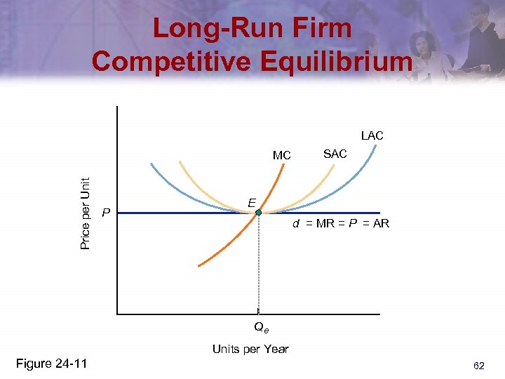Long-Run Firm Competitive Equilibrium LAC Price per Unit MC P SAC E d = MR = P = AR Qe Units per Year Figure 24 -11 62

Competitive Pricing: Marginal Cost Pricing n Marginal Cost Pricing – A system of pricing in which the price charged is equal to the opportunity cost to society of producing one more unit of the good or service in question 63

Competitive Pricing: Marginal Cost Pricing n Market Failure – A situation in which an unrestrained market operation leads to either too few or too many resources going to a specific economic activity 64

Issues and Applications: Full-Body Medical Scanning n Full-body CT scans can provide early detection of internal diseases. n In the late 1990’s, the price of the procedure was about $1, 500. n This price was well above the provider’s average cost. 65

Issues and Applications: Full-Body Medical Scanning n More firms entered the market of providing CT scans in response to the profit level. n In recent years, some physicians have recommended against the procedure. n The simultaneous increase in supply and decrease in demand has dropped the prevailing price to about $400, which allows the remaining firms to earn a normal profit. 66

Summary Discussion of Learning Objectives n The characteristics of a perfectly competitive market structure – Large number of buyers and sellers – Homogeneous product – No barriers to entry and exit – Buyers and sellers have equal access to information 67

Summary Discussion of Learning Objectives n How a perfectly competitive firm decides how much to produce – Economic profits are maximized when marginal cost equals marginal revenue above minimum average variable cost 68

Summary Discussion of Learning Objectives n The short-run supply curve of a perfectly competitive firm – The rising part of the marginal cost curve above minimum average variable cost n The equilibrium price in a perfectly competitive market – A price at which the total amount of output supplied by all firms is equal to the total amount of output demanded by all buyers 69

Summary Discussion of Learning Objectives n Incentives to enter or exit a perfectly competitive industry – Economic profits induce entry of new firms – Economic losses will induce firms to exit the industry 70

Summary Discussion of Learning Objectives n The long-run industry supply curve and constant-, increasing-, and decreasing-cost industries – The relationship between price and quantity after firms have been able to enter or exit the industry – Constant-cost industry • Horizontal long-run supply curve – Increasing-cost industry • Upward-sloping long-run supply curve – Decreasing-cost industry • Downward-sloping long-run supply curve 71

End of Chapter 24 Perfect Competition