Chapter 21 Theory of Consumer Choice Budget

Chapter 21 Theory of Consumer Choice

Budget Constraint: What the Consumer can Afford • Budget constraint – Limit on the consumption bundles that a consumer can afford • Trade-off between goods • Slope of the budget constraint • Rate at which the consumer can trade one good for the other • Change in the vertical distance • Divided by the change in the horizontal distance – Relative price of the two goods 2

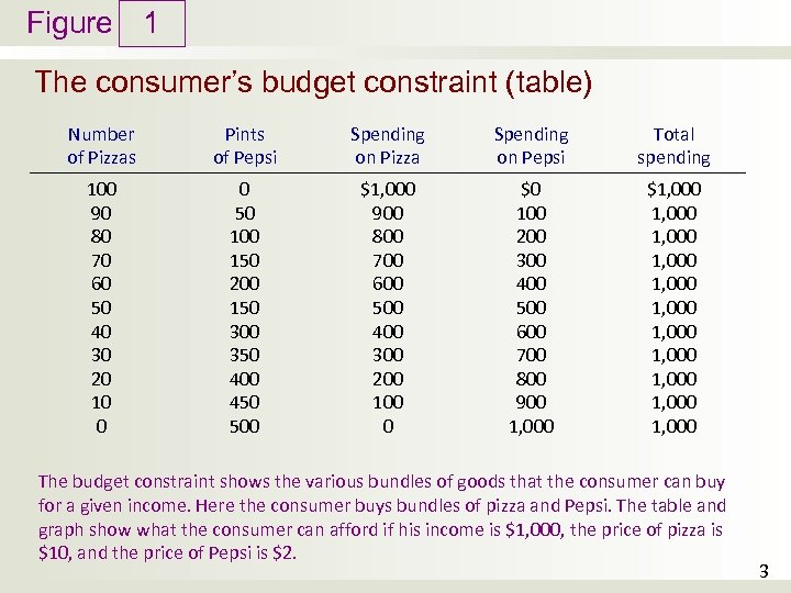
Figure 1 The consumer’s budget constraint (table) Number of Pizzas Pints of Pepsi Spending on Pizza Spending on Pepsi Total spending 100 90 80 70 60 50 40 30 20 10 0 0 50 100 150 200 150 300 350 400 450 500 $1, 000 900 800 700 600 500 400 300 200 100 0 $0 100 200 300 400 500 600 700 800 900 1, 000 $1, 000 1, 000 1, 000 The budget constraint shows the various bundles of goods that the consumer can buy for a given income. Here the consumer buys bundles of pizza and Pepsi. The table and graph show what the consumer can afford if his income is $1, 000, the price of pizza is $10, and the price of Pepsi is $2. 3

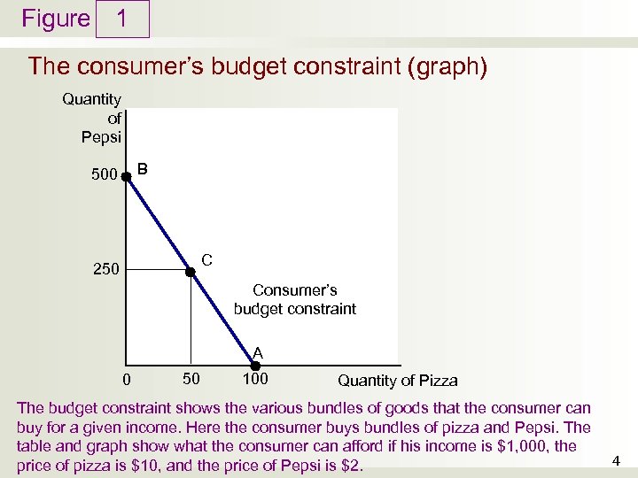
Figure 1 The consumer’s budget constraint (graph) Quantity of Pepsi B 500 C 250 Consumer’s budget constraint A 0 50 100 Quantity of Pizza The budget constraint shows the various bundles of goods that the consumer can buy for a given income. Here the consumer buys bundles of pizza and Pepsi. The table and graph show what the consumer can afford if his income is $1, 000, the price of pizza is $10, and the price of Pepsi is $2. 4

Preferences: What the Consumer Wants • Indifference curve – Shows consumption bundles that give the consumer the same level of satisfaction – Combinations of goods on the same curve • Same satisfaction • Slope of indifference curve – Marginal rate of substitution • Rate at which a consumer is willing to trade one good for another – Not the same at all points 5

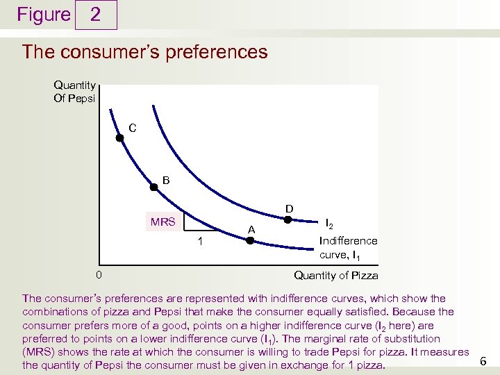
Figure 2 The consumer’s preferences Quantity Of Pepsi C B D MRS 1 0 A I 2 Indifference curve, I 1 Quantity of Pizza The consumer’s preferences are represented with indifference curves, which show the combinations of pizza and Pepsi that make the consumer equally satisfied. Because the consumer prefers more of a good, points on a higher indifference curve (I 2 here) are preferred to points on a lower indifference curve (I 1). The marginal rate of substitution (MRS) shows the rate at which the consumer is willing to trade Pepsi for pizza. It measures 6 the quantity of Pepsi the consumer must be given in exchange for 1 pizza.

Preferences: What the Consumer Wants • Four properties of indifference curves 1. Higher indifference curves are preferred to lower ones – Higher indifference curves – more goods 2. Indifference curves are downward sloping 3. Indifference curves do not cross 4. Indifference curves are bowed inward 7

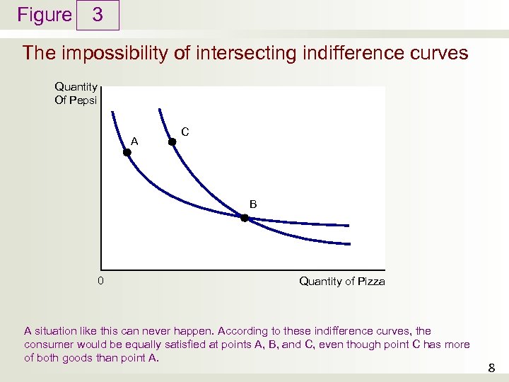
Figure 3 The impossibility of intersecting indifference curves Quantity Of Pepsi A C B 0 Quantity of Pizza A situation like this can never happen. According to these indifference curves, the consumer would be equally satisfied at points A, B, and C, even though point C has more of both goods than point A. 8

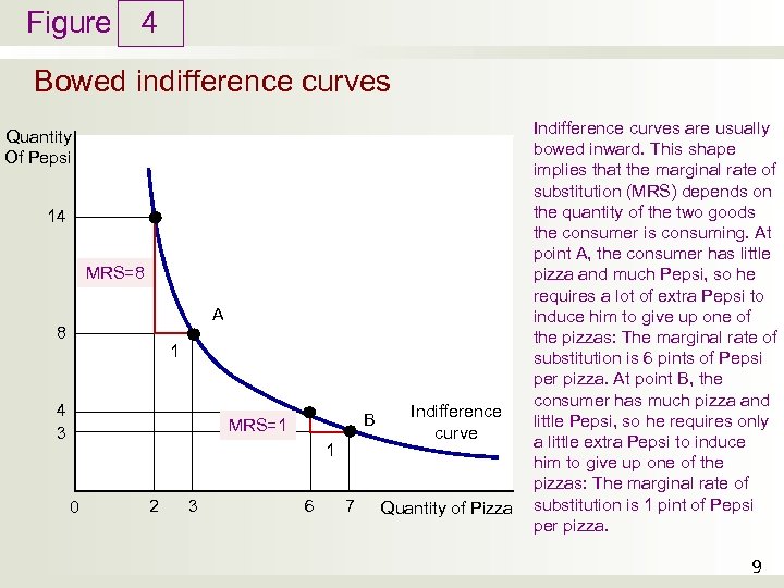
Figure 4 Bowed indifference curves Quantity Of Pepsi 14 MRS=8 A 8 1 4 3 B MRS=1 1 0 2 3 6 7 Indifference curve Quantity of Pizza Indifference curves are usually bowed inward. This shape implies that the marginal rate of substitution (MRS) depends on the quantity of the two goods the consumer is consuming. At point A, the consumer has little pizza and much Pepsi, so he requires a lot of extra Pepsi to induce him to give up one of the pizzas: The marginal rate of substitution is 6 pints of Pepsi per pizza. At point B, the consumer has much pizza and little Pepsi, so he requires only a little extra Pepsi to induce him to give up one of the pizzas: The marginal rate of substitution is 1 pint of Pepsi per pizza. 9

Preferences: What the Consumer Wants • Two extreme examples of indifference curves • Perfect substitutes – Two goods with straight-line indifference curves – Marginal rate of substitution – constant • E. g. : nickels and dimes bundles • Perfect complements – Two goods with right-angle indifference curves • E. g. : right shoe and left shoe bundle 10

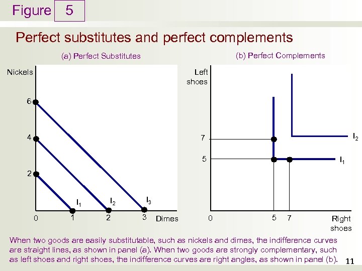
Figure 5 Perfect substitutes and perfect complements (b) Perfect Complements (a) Perfect Substitutes Left shoes Nickels 6 4 I 2 7 5 I 1 2 I 1 0 1 I 2 2 I 3 3 Dimes 0 5 7 Right shoes When two goods are easily substitutable, such as nickels and dimes, the indifference curves are straight lines, as shown in panel (a). When two goods are strongly complementary, such as left shoes and right shoes, the indifference curves are right angles, as shown in panel (b). 11

Optimization: What the Consumer Chooses • The consumer’s optimal choices • Optimum – Point where indifference curve and budget constraint touch – Best combination of goods available to the consumer – Slope of indifference curve • Equals slope of budget constraint • Marginal rate of substitution = relative price 12

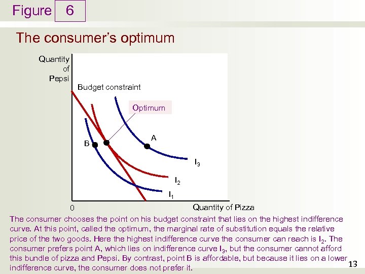
Figure 6 The consumer’s optimum Quantity of Pepsi Budget constraint Optimum B A I 3 I 2 I 1 Quantity of Pizza 0 The consumer chooses the point on his budget constraint that lies on the highest indifference curve. At this point, called the optimum, the marginal rate of substitution equals the relative price of the two goods. Here the highest indifference curve the consumer can reach is I 2. The consumer prefers point A, which lies on indifference curve I 3, but the consumer cannot afford this bundle of pizza and Pepsi. By contrast, point B is affordable, but because it lies on a lower 13 indifference curve, the consumer does not prefer it.

Optimization: What the Consumer Chooses • How changes in income affect the consumer’s choices • Higher income – Consumer can afford more of both goods – Shifts the budget constraint outward – New optimum 14

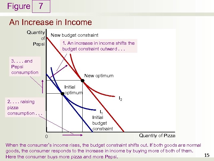
Figure 7 An Increase in Income Quantity of Pepsi New budget constraint 1. An increase in income shifts the budget constraint outward. . . 3. . and Pepsi consumption New optimum Initial optimum I 2 2. . raising pizza consumption. . . I 1 Initial budget constraint 0 Quantity of Pizza When the consumer’s income rises, the budget constraint shifts out. If both goods are normal goods, the consumer responds to the increase in income by buying more of both of them. 15 Here the consumer buys more pizza and more Pepsi.

Optimization: What the Consumer Chooses • How changes in income affect the consumer’s choices • Normal good – Good for which an increase in income raises the quantity demanded • Inferior good – Good for which an increase in income reduces the quantity demanded 16

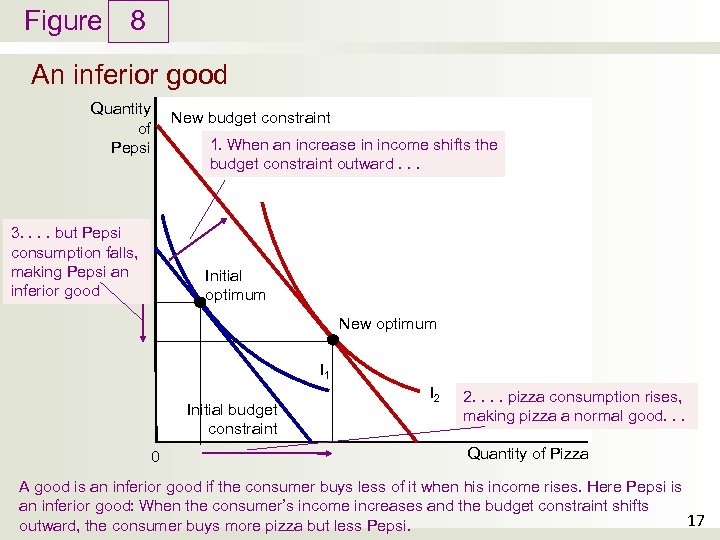
Figure 8 An inferior good Quantity of Pepsi New budget constraint 1. When an increase in income shifts the budget constraint outward. . . 3. . but Pepsi consumption falls, making Pepsi an inferior good Initial optimum New optimum I 1 Initial budget constraint 0 I 2 2. . pizza consumption rises, making pizza a normal good. . . Quantity of Pizza A good is an inferior good if the consumer buys less of it when his income rises. Here Pepsi is an inferior good: When the consumer’s income increases and the budget constraint shifts 17 outward, the consumer buys more pizza but less Pepsi.

Optimization: What the Consumer Chooses • How changes in prices affect the consumer’s choices • Price of one good falls – Rotates the budget constraint outward • Steeper slope • Change in relative price – Income effect – Substitution effect 18

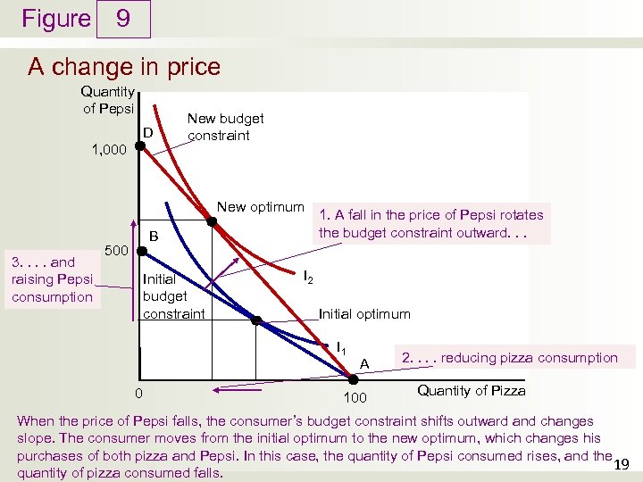
Figure 9 A change in price Quantity of Pepsi D 1, 000 New budget constraint New optimum 3. . and raising Pepsi consumption B 500 Initial budget constraint 1. A fall in the price of Pepsi rotates the budget constraint outward. . . I 2 Initial optimum I 1 0 A 100 2. . reducing pizza consumption Quantity of Pizza When the price of Pepsi falls, the consumer’s budget constraint shifts outward and changes slope. The consumer moves from the initial optimum to the new optimum, which changes his purchases of both pizza and Pepsi. In this case, the quantity of Pepsi consumed rises, and the 19 quantity of pizza consumed falls.

Optimization: What the Consumer Chooses • Income effect – Change in consumption – When a price change moves the consumer • To a higher or lower indifference curve • Substitution effect – Change in consumption – When a price change moves the consumer • Along a given indifference curve • To a point with a new marginal rate of substitution 20

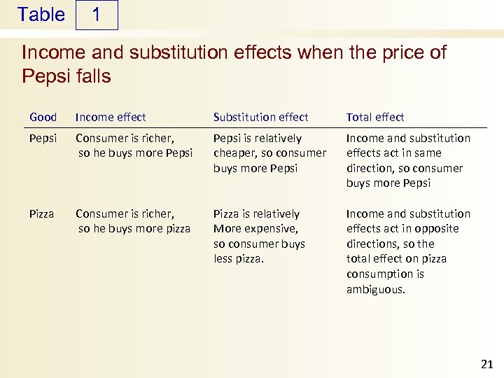
Table 1 Income and substitution effects when the price of Pepsi falls Good Income effect Substitution effect Total effect Pepsi Consumer is richer, so he buys more Pepsi is relatively cheaper, so consumer buys more Pepsi Income and substitution effects act in same direction, so consumer buys more Pepsi Pizza Consumer is richer, so he buys more pizza Pizza is relatively More expensive, so consumer buys less pizza. Income and substitution effects act in opposite directions, so the total effect on pizza consumption is ambiguous. 21

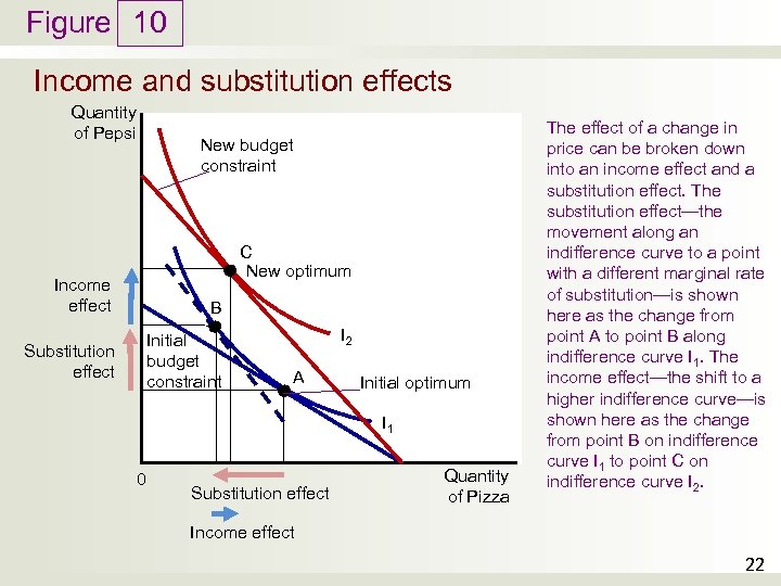
Figure 10 Income and substitution effects Quantity of Pepsi New budget constraint C New optimum Income effect B Initial budget constraint Substitution effect I 2 A Initial optimum I 1 0 Substitution effect Quantity of Pizza The effect of a change in price can be broken down into an income effect and a substitution effect. The substitution effect—the movement along an indifference curve to a point with a different marginal rate of substitution—is shown here as the change from point A to point B along indifference curve I 1. The income effect—the shift to a higher indifference curve—is shown here as the change from point B on indifference curve I 1 to point C on indifference curve I 2. Income effect 22

Optimization: What the Consumer Chooses • Deriving the demand curve – Quantity demanded of a good for any given price – Initial optimum point • Initial price of the good • Initial quantity of the good – A change in price of the good (new price) • New optimum quantity 23

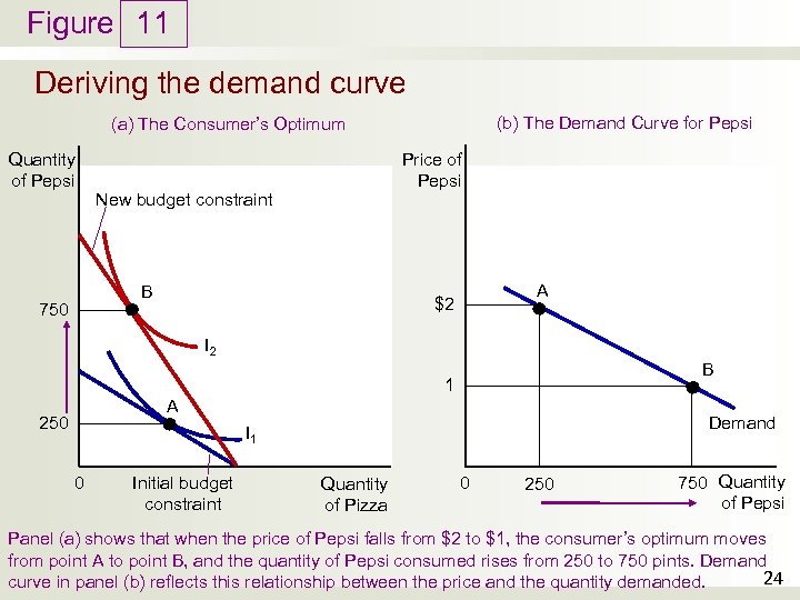
Figure 11 Deriving the demand curve (b) The Demand Curve for Pepsi (a) The Consumer’s Optimum Quantity of Pepsi Price of Pepsi New budget constraint B 750 A $2 I 2 B 1 A 250 Demand I 1 0 Initial budget constraint Quantity of Pizza 0 250 750 Quantity of Pepsi Panel (a) shows that when the price of Pepsi falls from $2 to $1, the consumer’s optimum moves from point A to point B, and the quantity of Pepsi consumed rises from 250 to 750 pints. Demand 24 curve in panel (b) reflects this relationship between the price and the quantity demanded.

Three Applications • Do all demand curves slope downward? • Law of demand – When the price of a good rises, people buy less of it • Downward slope of the demand curve • Giffen good – An increase in the price of the good raises the quantity demanded • Income effect dominates the substitution effect • Demand curve – slopes upward 25

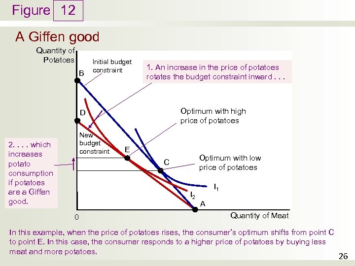
Figure 12 A Giffen good Quantity of Potatoes B Initial budget constraint 1. An increase in the price of potatoes rotates the budget constraint inward. . . Optimum with high price of potatoes D New budget constraint 2. . which increases potato consumption if potatoes are a Giffen good. E Optimum with low price of potatoes C I 2 0 I 1 A Quantity of Meat In this example, when the price of potatoes rises, the consumer’s optimum shifts from point C to point E. In this case, the consumer responds to a higher price of potatoes by buying less meat and more potatoes. 26

The search for Giffen goods • Potatoes - Giffen good during the Irish potato famine of the 19 th century – Price of potatoes rose • Large income effect • People – cut back on the luxury of meat • Buy more of the staple food of potatoes • Chinese province of Hunan, rice – Poor households exhibited Giffen behavior • Lower price of rice (with subsidy voucher) – Households - reduce their consumption of rice • Higher price of rice (remove the subsidy) – Households – increase consumption of rice 27

Three Applications • How do wages affect labor supply? • Trade-off between leisure and consumption • Bundle of goods: leisure and work – Given wage – Budget constraint – Optimum 28

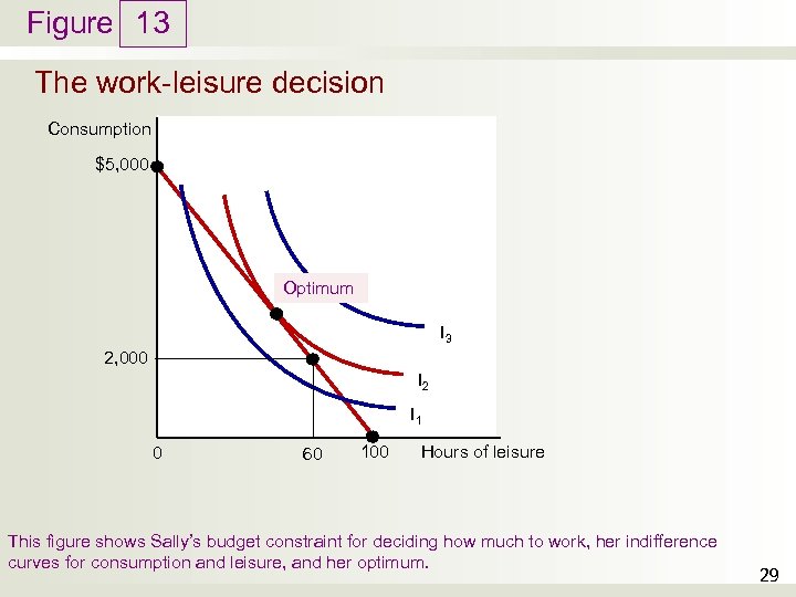
Figure 13 The work-leisure decision Consumption $5, 000 Optimum I 3 2, 000 I 2 I 1 0 60 100 Hours of leisure This figure shows Sally’s budget constraint for deciding how much to work, her indifference curves for consumption and leisure, and her optimum. 29

Three Applications • How do wages affect labor supply? • Increase in wage – Budget constraint shifts outward • Steeper • New optimum – If enjoy less leisure • Work more • Upward-sloping labor supply curve • Substitution effect dominates 30

Three Applications • How do wages affect labor supply? • Increase in wage – Budget constraint shifts outward • Steeper • New optimum – If enjoy more leisure • Work less • Backward-sloping labor supply curve • Income effect dominates 31

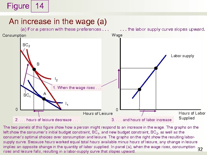
Figure 14 An increase in the wage (a). . . the labor supply curve slopes upward. (a) For a person with these preferences. . . Wage Consumption BC 2 Labor supply B I 2 1. When the wage rises. . . BC 1 A I 1 0 2. . hours of leisure decrease. . . Hours of Leisure 0 3. . and hours of labor increase Hours of Labor Supplied The two panels of this figure show a person might respond to an increase in the wage. The graphs on the left show the consumer’s initial budget constraint, BC 1, and new budget constraint, BC 2, as well as the consumer’s optimal choices over consumption and leisure. The graphs on the right show the resulting laborsupply curve. Because hours worked equal total hours available minus hours of leisure, any change in leisure implies an opposite change in the quantity of labor supplied. In panel (a), when the wage rises, consumption 32 rises and leisure falls, resulting in a labor-supply curve that slopes upward.

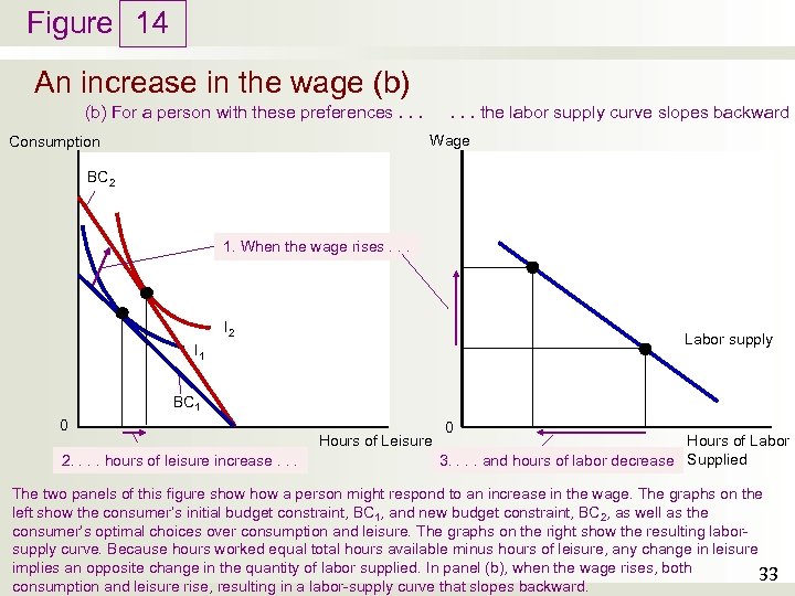
Figure 14 An increase in the wage (b). . . the labor supply curve slopes backward (b) For a person with these preferences. . . Wage Consumption BC 2 1. When the wage rises. . . I 2 Labor supply I 1 BC 1 0 2. . hours of leisure increase. . . Hours of Leisure 0 Hours of Labor 3. . and hours of labor decrease Supplied The two panels of this figure show a person might respond to an increase in the wage. The graphs on the left show the consumer’s initial budget constraint, BC 1, and new budget constraint, BC 2, as well as the consumer’s optimal choices over consumption and leisure. The graphs on the right show the resulting laborsupply curve. Because hours worked equal total hours available minus hours of leisure, any change in leisure implies an opposite change in the quantity of labor supplied. In panel (b), when the wage rises, both 33 consumption and leisure rise, resulting in a labor-supply curve that slopes backward.

Income effects on labor supply: historical trends, lottery winners, & Carnegie conjecture • Labor- supply curve, over long periods – Slope backward • A hundred years ago – People worked six days a week • Today – Five-day workweeks – Length of the workweek has been falling – Wage of the typical worker (adjusted for inflation) has been rising 34

Income effects on labor supply: historical trends, lottery winners, & Carnegie conjecture • Explanation: Advances in technology – Higher worker productivity – Increase in demand for labor • • • Higher equilibrium wages Greater reward for working Income effect dominates substitution effect More leisure Less work 35

Income effects on labor supply: historical trends, lottery winners, & Carnegie conjecture • Winners of lotteries – Large increase in incomes – Large outward shifts in budget constraints • Same slope • No substitution effect – Income effect on labor supply • Substantial • People who win the lottery – tend to quit their jobs 36

Income effects on labor supply: historical trends, lottery winners, & Carnegie conjecture • Andrew Carnegie, 19 th century – “The parent who leaves his son enormous wealth generally deadens the talents and energies of the son, and tempts him to lead a less useful and less worthy life than he otherwise would” – Income effect on labor supply – substantial 37

Three Applications • How do interest rates affect household saving? • Income decision – Consume today or Save for future • Bundle of goods – Consumption today and Consumption in the future – Relative price = interest rates – Optimum: Budget constraint & Indifference curves 38

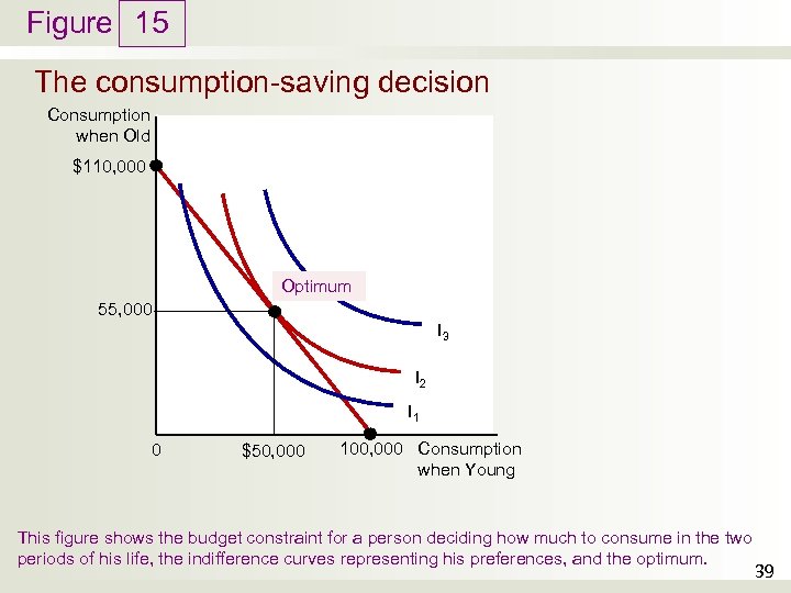
Figure 15 The consumption-saving decision Consumption when Old $110, 000 Optimum 55, 000 I 3 I 2 I 1 0 $50, 000 100, 000 Consumption when Young This figure shows the budget constraint for a person deciding how much to consume in the two periods of his life, the indifference curves representing his preferences, and the optimum. 39

Three Applications • How do interest rates affect household saving? • Increase in interest rates – Budget constraint – shifts outward • Steeper – Consumption in the future – rises – If consume less today • Substitution effect dominates; Save more – If consume more today • Income effect dominates; Save less 40

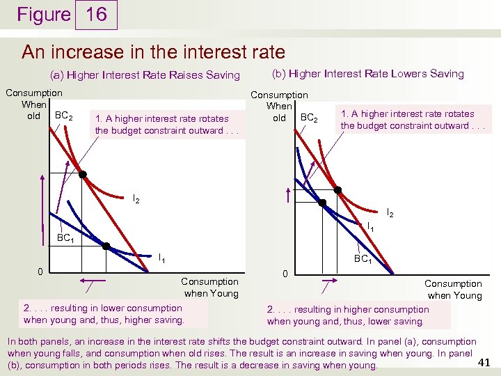
Figure 16 An increase in the interest rate (a) Higher Interest Rate Raises Saving Consumption When old BC 2 1. A higher interest rate rotates the budget constraint outward. . . (b) Higher Interest Rate Lowers Saving Consumption When old BC 2 1. A higher interest rate rotates the budget constraint outward. . . I 2 I 1 BC 1 I 1 0 BC 1 Consumption when Young 2. . resulting in lower consumption when young and, thus, higher saving. 0 Consumption when Young 2. . resulting in higher consumption when young and, thus, lower saving. In both panels, an increase in the interest rate shifts the budget constraint outward. In panel (a), consumption when young falls, and consumption when old rises. The result is an increase in saving when young. In panel 41 (b), consumption in both periods rises. The result is a decrease in saving when young.