Chapter 20 Introduction to Commercial Mortgage Backed Securities

Chapter 20: Introduction to Commercial Mortgage Backed Securities (CMBS)

Chapter Focus: • The basic outlines of the US CMBS industry, including the typical structure of CMBS products and the role played by rating agencies. • What is meant by “tranching”, and how this is used to concentrate and stratify the default risk in CMBS. • What determines the market yields of CMBS, and why these yields may differ from those of corporate bonds.

Chapter Outline 20. 1. What are CMBS? . . . 20. 1. 1 A brief history: The birth of an industry 20. 1. 2: Conduits, Seasoned loans, and Risk-based capital requirements 20. 1. 3 The magnitude of the CMBS industry 20. 2 CMBS structure: Tranching & Subordination 20. 2. 1 A simple numerical example of tranching 20. 2. 2 Allocating the credit losses 20. 3 CMBS Rating and Yields 20. 3. 1 Bond credit rating 20. 3. 2 Credit rating & CMBS structure 20. 3. 3 Rating CMBS tranches 20. 3. 4 Yield spreads and the capital market 20. 3. 5 CMBS versus corporate bond spreads

First, A Prequel… Residential Mortgage Backed Securities (RMBS) RMBS were securitized before CMBS, and much of the basic technology was perfected in the RMBS market. In fact, the antecedents of the RMBS market lie in the development of the home mortgage secondary market, which dates from the housing policy of the Roosevelt administration in the 1930 s. . .

Promotion of 2 ndary mortgage market A “mortgage” (IOU contract + mortgage deed) is a secured promise to pay a stream of future cash flows. It is thus a capital asset. In principle, it can be traded from one owner to another. For example, original issuing bank sells the mortgage to a life insurance company or pension fund. (Bank has ST liabilities it needs to match with ST assets, but mortg is LT asset; LIC or PF has LT liabilities it needs to match with LT assets. ) Issuing institution then can make a new loan (with the cash from loan sale). Issuing institution’s expertise (and therefore profit-making ability) lies in mortgage issuance. The more loans it can issue, the more profit it can make.

Original issuance of mortgage = Primary mortgage mkt. Subsequent trading of mortgage = Secondary mortg mkt. Well-functioning 2 ndary mkt promotes efficient allocation of capital. . . Phoenix Pittsburgh Young people move to Phnx from Pgh, leaving: • Lots of young peo w no capital but good income prospects needing houses. • Local mortg mkt w high demand, low supply of capital. High in Phoenix Making it hard for young peo to afford houses they need. What will interest rates be like? • Old peo w lots capital & houses all paid for, needing investmt income. • Local mortg mkt w low demand, high supply of capital. Low in Pittsburgh Making it hard for old peo to get investmt income they need. Enter: a 2 ndary market for mortgages. . .

What will happen? . . . Phoenix Pittsburgh Capital will flow in the direction of the people Driving mortg prices up (int. rates down) in Phoenix. Making it easier for young peo to afford houses. Pgh investors will sell Pgh mortgages, buy Phoenix mortgages Driving mortg prices down (int. rates up) in Pgh. Making it easier for old peo to obtain investmt income. With an integrated, national mortgage market, interest rates will be the same all across the country.

Despite its obvious benefits, this did not happen naturally in our capitalist system. Why? Primary mortg mkt requires local expertise (hse quality, nghd quality, income potential: familiarity with default risk). 2 ndary mortg mkt is full of conservative investors who lack local expertise. They don’t know how to judge the default risk, but they do know that they don’t want it. Hence: 2 ndary mkt has no liquidity (no buyers, i. e. , no investors). To create a 2 ndary mortg mkt you need: Mortgage Default Insurance Enter: FHA & FNMA (1930 s), later VA, FHLMC & GNMA.

At first, Govt agencies (FNMA, FHLMC) made the secondary market by themselves. They bought mortgages from issuers, and merely held these mortgages in their own portfolios, or sold them as whole loans with their mortgage insurance attached. This was a limited source of capital. Then, securitization developed (GNMA, etc) in 1970 s. “Pass-Through” securities were the first to be developed: • Pool a bunch of individual mortgages together, • Issue undifferentiated securities (small homogeneous units) on the pool, • Issuing agency provides payment guarantee (removes default risk), • Each unit receives its pro rata share of all the cash flow coming into the pool, Including CF from: • Interest payments • Principal amortization payments • Prepayments of loans (payment of outstanding loan balance to pay off mortgage) Securitization greatly expanded the source of capital to include the vast bond market.

This is a great system, greatly improved the efficiency of the housing market. System has been copied by other countries. Greatly enhanced the quant & qual of U. S. housing stock. Greatly promoted home ownership (and later rental housing stock too, via GNMA, & FNMA/FHLMC multi-family housing programs). One important result is standardized (“mass production”) residential mortgage products (more on this later). FNMA, FHLMC now private corporations (since 1968), traded on NYSE. (Still chartered by Fed. Govt. GNMA remains Govt owned. ) Most mortg insurance is now provided by private firms, but FHA & VA are still active, esp. for 1 st-time & low-income homebuyers.

Problem: Pass-through securities have “prepayment risk”: Investors do not know exact duration of the security, because: Residential mortgages are “callable”: Subject to pay off by borrower before maturity. Like callable corporate bonds, only more problematical because: • Many borrowers & loans in underlying pool heterogeneous prepayment behavior: Some loans will prepay early, some late, etc. • Prepayment behavior governed not just by financial (interest rate) factors, but also by demographic factors (“non-financial termination”: “due-on-sale” clause terminations due to upward mobility, migration, household formation, birth, divorce, death, etc. , even if interest rates are higher than contract rate on old loan). Many bond investors do not like prepayment risk. They need relative certainty of maturity (or duration) of their bond investments (e. g. , to match maturity of liabilities, to implement “immunization” investment strategies).

Solution: RMBS “derivatives” : • “Collateralized Mortgage Obligations (CMOs) • Interest-Only (IO) and Principle-Only (PO) “Strips” Developed in the 1980 s. Greatly expanded the market for MBS, thereby further increasing the pool of capital available to mortgages. Resulted in (or from) the development of financial engineering technology (“tranching”, “stripping”) that subsequently was instrumental in the development of the CMBS market in the 1990 s.

In the classical CMO, different classes of securities (called “tranches”) are defined based on the underlying pass-thru pool, Based on priority of receipt of payments of principal. This “sequential payment” assignment results in classes of securities whose durations are: • Differentiated, • More precise within each tranche. How this works is best seen by a simple numerical example…

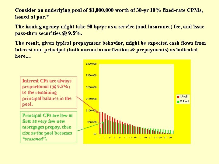
Consider an underlying pool of $1, 000 worth of 30 -yr 10% fixed-rate CPMs, issued at par. * The issuing agency might take 50 bp/yr as a service (and insurance) fee, and issue pass-thru securities @ 9. 5%. The result, given typical prepayment behavior, might be expected cash flows from interest and principal (both normal amortization & prepayments) as indicated here… Interest CFs are always proportional (@ 9. 5%) to the remaining principal balance in the pool. Principal CFs are low at first as very few new mortgages prepay, then rise as the pool becomes “seasoned”.

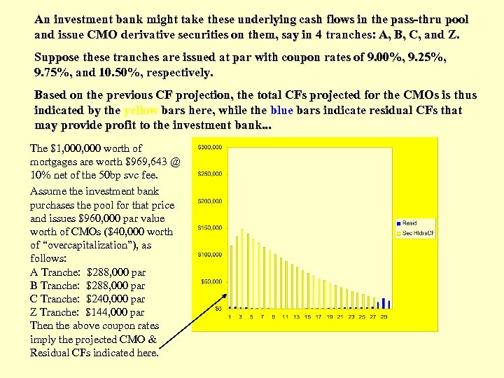
An investment bank might take these underlying cash flows in the pass-thru pool and issue CMO derivative securities on them, say in 4 tranches: A, B, C, and Z. Suppose these tranches are issued at par with coupon rates of 9. 00%, 9. 25%, 9. 75%, and 10. 50%, respectively. Based on the previous CF projection, the total CFs projected for the CMOs is thus indicated by the yellow bars here, while the blue bars indicate residual CFs that may provide profit to the investment bank. . . The $1, 000 worth of mortgages are worth $969, 643 @ 10% net of the 50 bp svc fee. Assume the investment bank purchases the pool for that price and issues $960, 000 par value worth of CMOs ($40, 000 worth of “overcapitalization”), as follows: A Tranche: $288, 000 par B Tranche: $288, 000 par C Tranche: $240, 000 par Z Tranche: $144, 000 par Then the above coupon rates imply the projected CMO & Residual CFs indicated here.

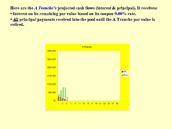
Here are the A Tranche’s projected cash flows (interest & principal). It receives: • Interest on its remaining par value based on its coupon 9. 00% rate. • All principal payments received into the pool until the A Tranche par value is retired.

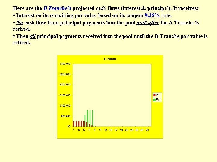
Here are the B Tranche’s projected cash flows (interest & principal). It receives: • Interest on its remaining par value based on its coupon 9. 25% rate. • No cash flow from principal payments into the pool until after the A Tranche is retired. • Then all principal payments received into the pool until the B Tranche par value is retired.

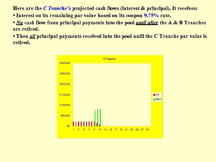
Here are the C Tranche’s projected cash flows (interest & principal). It receives: • Interest on its remaining par value based on its coupon 9. 75% rate. • No cash flow from principal payments into the pool until after the A & B Tranches are retired. • Then all principal payments received into the pool until the C Tranche par value is retired.

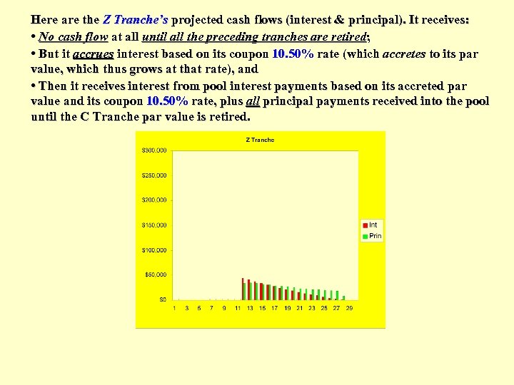
Here are the Z Tranche’s projected cash flows (interest & principal). It receives: • No cash flow at all until all the preceding tranches are retired; • But it accrues interest based on its coupon 10. 50% rate (which accretes to its par value, which thus grows at that rate), and • Then it receives interest from pool interest payments based on its accreted par value and its coupon 10. 50% rate, plus all principal payments received into the pool until the C Tranche par value is retired.

As noted, this “slicing & dicing” of the underlying pool cash flows (the sequential payment “waterfall”) differentiates & concentrates the duration of the pool’s cash flows, thereby reducing prepayment uncertainty within each tranche. Within each tranche, the time over which principal payments are received is narrowed, creating a more “bullet-like” cash flow pattern, more like that of classical corporate & Govt bonds. The result is that the sum of the parts is worth more than the whole, because the needs of heterogeneous investors in the bond market (with different “preferred habitats”) are better served. Concept check: Why did the tranches have the rising market yields noted previously (9. 00%, 9. 25%, 9. 75%, 10. 50%)? . . .

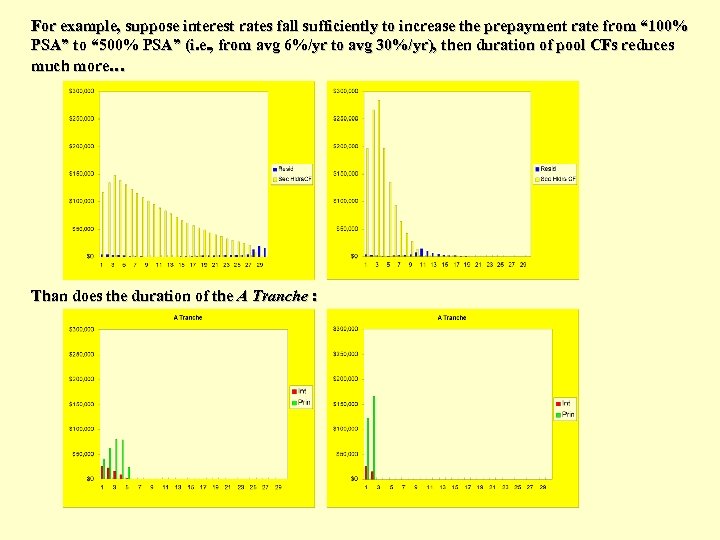
For example, suppose interest rates fall sufficiently to increase the prepayment rate from “ 100% PSA” to “ 500% PSA” (i. e. , from avg 6%/yr to avg 30%/yr), then duration of pool CFs reduces much more… Than does the duration of the A Tranche :

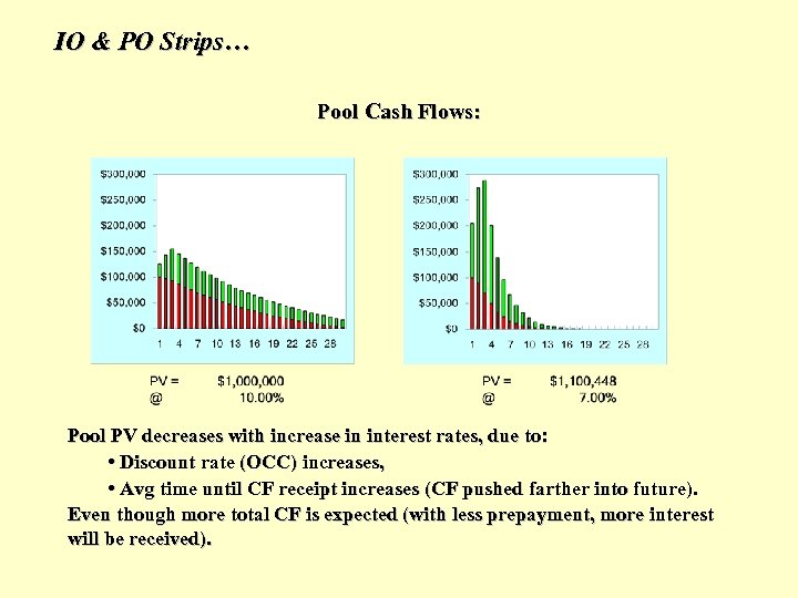
IO & PO Strips… Pool Cash Flows: Pool PV decreases with increase in interest rates, due to: • Discount rate (OCC) increases, • Avg time until CF receipt increases (CF pushed farther into future). Even though more total CF is expected (with less prepayment, more interest will be received).

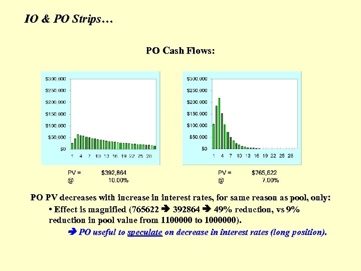
IO & PO Strips… PO Cash Flows: PO PV decreases with increase in interest rates, for same reason as pool, only: • Effect is magnified (765622 392864 49% reduction, vs 9% reduction in pool value from 1100000 to 1000000). PO useful to speculate on decrease in interest rates (long position).

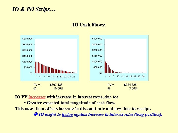
IO & PO Strips… IO Cash Flows: IO PV increases with increase in interest rates, due to: • Greater expected total magnitude of cash flow, This more than offsets increase in discount rate and avg time to receipt. IO useful to hedge against increase in interest rates (long position).

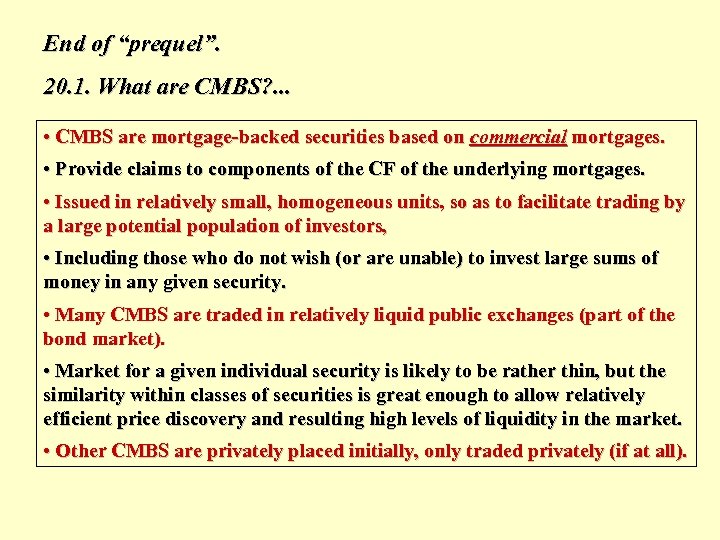
End of “prequel”. 20. 1. What are CMBS? . . . • CMBS are mortgage-backed securities based on commercial mortgages. • Provide claims to components of the CF of the underlying mortgages. • Issued in relatively small, homogeneous units, so as to facilitate trading by a large potential population of investors, • Including those who do not wish (or are unable) to invest large sums of money in any given security. • Many CMBS are traded in relatively liquid public exchanges (part of the bond market). • Market for a given individual security is likely to be rather thin, but the similarity within classes of securities is great enough to allow relatively efficient price discovery and resulting high levels of liquidity in the market. • Other CMBS are privately placed initially, only traded privately (if at all).

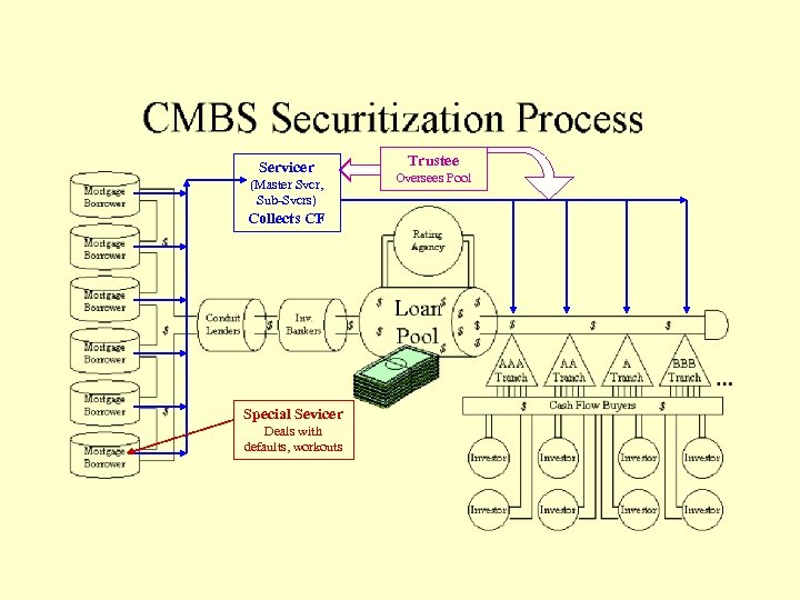
Servicer (Master Svcr, Sub-Svcrs) Collects CF Special Sevicer Deals with defaults, workouts Trustee Oversees Pool

20. 1. 1 A brief history: The birth of an industry. . . • Resolution Trust Corporation (RTC), Financial Institutions Reform, Recovery and Enforcement Act of 1989 (FIRREA): • RTC (Federal Govt Corp) set up to liquidate the loan portfolios of thrifts and banks that had failed in the commercial property crash of the late 1980 s. RTC had to sell large quantities of commercial mortgages, quickly. • Traditional private instl sources of R. E. capital not available at that time (they were “crashing and burning” due to 80 s R. E. finance binge). But bond mkt on Wall St was thriving, spent the 1970 s and 80 s cutting its teeth on derivatives based on residential MBS, had developed procedures useful for securitizing large pools of mortgages (e. g. , “tranching”). • Key players and investors in the public capital markets perceived in the early 1990 s that the commercial property market had “over-shot”, fallen too far relative to fundamental value, and it was also obvious that the RTC was under great political pressure to sell assets quickly. “Grave-dancers” and bargain-hunters provided a market, helped the RTC to give birth to the CMBS market.

Key was devlpt by bond-rating agencies of the ability to rate the default-risk of CMBS tranches: Traditional Bond Credit Rating Labels Applied to CMBS Recall heterogeneity of investor population… • Bond mkt full of “passive investors” (lack time, resources, expertise to assess risk of individual bonds). Won’t invest w/out a reliable measure of default risk. • As with original devlpt of the 2 ndary mkt for residential mortgages in the 1930 s-50 s, a CMBS market could not develop until the investment industry figured out a way to apply traditional bond mkt credit risk ratings to CMBS. • With RMBS this problem had been solved by the use of mortgage insurance and pool insurance. • With CMBS it was necessary for bond rating agencies and investmt banks on Wall St to learn how to quantify the default risk of commercial mortgages. • This was done via sequential payment and sequential default assignment in the tranching of the securities issued from the CMBS pool. • When a CMBS tranche obtains a bond rating, investors who know little or nothing about commercial real estate feel comfortable working under the assumption that the default risk of that tranche is very similar to the default risk of any other bond with the same rating. • This vastly expands the pool of potential investors and makes the public market for CMBS viable.

20. 1. 2: Conduits, Seasoned loans, and Risk-based capital requirements Two types of loans in CMBS pool at time of IPO: • “Conduit” loans, • “Seasoned” loans. Conduit loans: New loans, issued with intent of being placed into a CMBS pool. Seasoned loans: Old loans, originally issued by a “portfolio lender”. Default risk and prepayment characteristics of new & old loans may differ, hence credit risk assessment must keep this difference in mind. Conduit lenders include: • Commercial banks, • Investment banks, • Mortgage banks, • Life Insurance Companies.

Traditionally commercial mortgages were almost entirely issued to be held in portfolio, as there was no major secondary market. Major portfolio lenders were (and are): • Life Insurance Companies (LICs) • Pension Funds (PFs) Why do you suppose these were the major types of lenders? Why would a portfolio lender such as a LIC want to sell its old loans into a CMBS pool? • During the 1990 s one reason was the establishment of new “risk-based capital requirements” (RBC) for depository institutions and life insurance companies. • RBC requirements make it necessary for banks and insurance companies to retain a greater amount of equity backing for investment in types of assets that are viewed as more risky. • RBC requirements view commercial mortgages in the form of whole loans as being more risky than good quality debt securities. Such loans could be sold into the CMBS market, and the proceeds of such a sale could be used to buy CMBS securities that had much lower RBC requirements than the original whole loan. (Tranching was a major means to accomplish this trick. ) • e. g. , Suppose for every $1 of equity a LIC could hold $20 worth of whole commercial mortgages, or $30 worth of investment grade rated bonds (including such CMBS tranches). The LIC can obtain greater leverage by selling mortgages into CMBS.

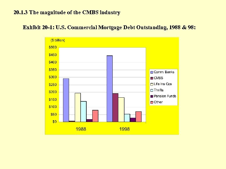
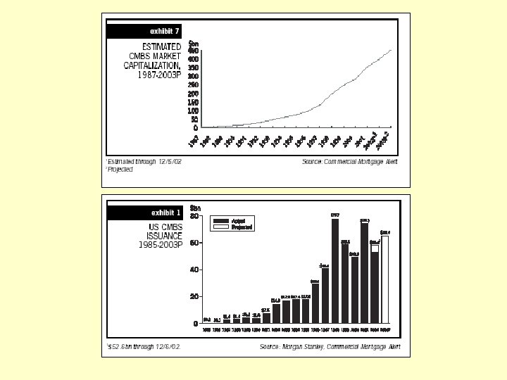
20. 1. 3 The magnitude of the CMBS industry Exhibit 20 -1: U. S. Commercial Mortgage Debt Outstanding, 1988 & 98:

Public market has gained share over time Mortgage market shares 42% 41% 3/31/91 3/31/01 21% 15% 13% 12% 11% 12% 8% 6% th e O na nc e C o. AB S r 1% 1% Fi io Pe ns nc ur a In s n e C Fu nd s o. t. In s s Sa vi ng ci er m om 3% 6% 4% C G ov er nm en t al En tit i Ba nk s es 4% Source: Federal Reserve Board Flow of Funds How far will it go? . . .

20. 2 CMBS structure: Tranching & Subordination Tranching cash flow claim priority involves two primary dimensions: • Loan Retirement. Duration, Int. Rate Risk. • Credit Losses. Default Risk. In CMBS it is usually the default risk dimension that is most important (most comm. mortgs have “prepayment protection”). The opposite is true in RMBS, where duration is the prime concern, due to the greater prepayment risk in residential loans (RMBS pools have “default protection”). Also, often an “IO” class is “stripped” off of the other securities (e. g. , from the excess of pool loan coupon interest over the A-Tranche coupon interest).

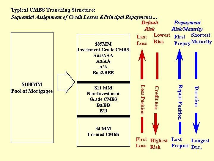
Typical CMBS Tranching Structure: Sequential Assignment of Credit Losses &Principal Repayments… Default Risk Last Lowest Loss Risk $85 MM Prepayment Risk/Maturity First Shortest Prepay Maturity Investment Grade CMBS Aaa/AAA Aa/AA A/A Baa 2/BBB Duration Repmt Position $4 MM Unrated CMBS Credit Risk $11 MM Non-Investment Grade CMBS Ba/BB B/B Loss Position $100 MM Pool of Mortgages First Highest Last Longest Loss Risk Prepmt Dur.

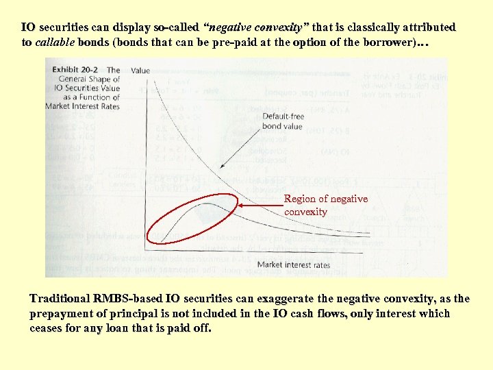
IO securities can display so-called “negative convexity” that is classically attributed to callable bonds (bonds that can be pre-paid at the option of the borrower)… Region of negative convexity Traditional RMBS-based IO securities can exaggerate the negative convexity, as the prepayment of principal is not included in the IO cash flows, only interest which ceases for any loan that is paid off.

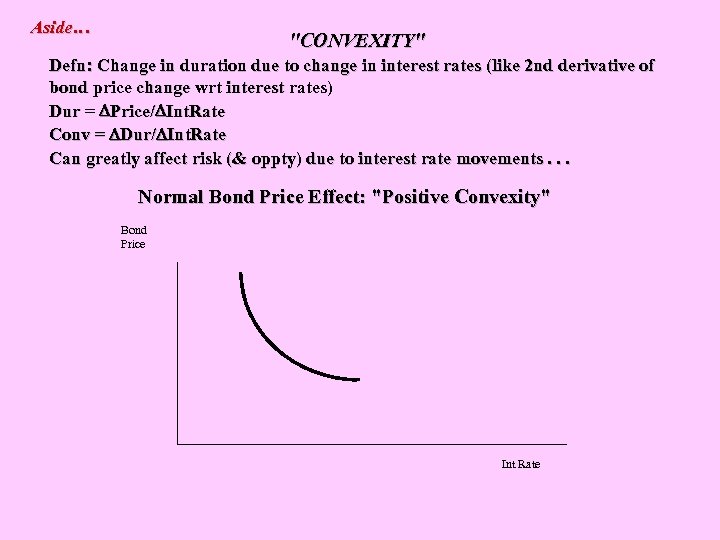
Aside… "CONVEXITY" Defn: Change in duration due to change in interest rates (like 2 nd derivative of bond price change wrt interest rates) Dur = Price/ Int. Rate Conv = Dur/ Int. Rate Can greatly affect risk (& oppty) due to interest rate movements. . . Normal Bond Price Effect: "Positive Convexity" Bond Price Int Rate

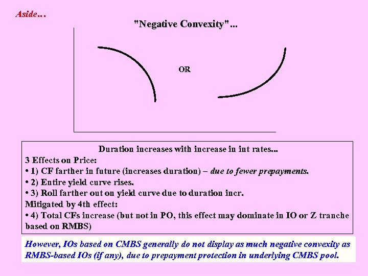
Aside… "Negative Convexity". . . OR Duration increases with increase in int rates. . . 3 Effects on Price: • 1) CF farther in future (increases duration) – due to fewer prepayments. • 2) Entire yield curve rises. • 3) Roll farther out on yield curve due to duration incr. Mitigated by 4 th effect: • 4) Total CFs increase (but not in PO, this effect may dominate in IO or Z tranche based on RMBS) However, IOs based on CMBS generally do not display as much negative convexity as RMBS-based IOs (if any), due to prepayment protection in underlying CMBS pool.

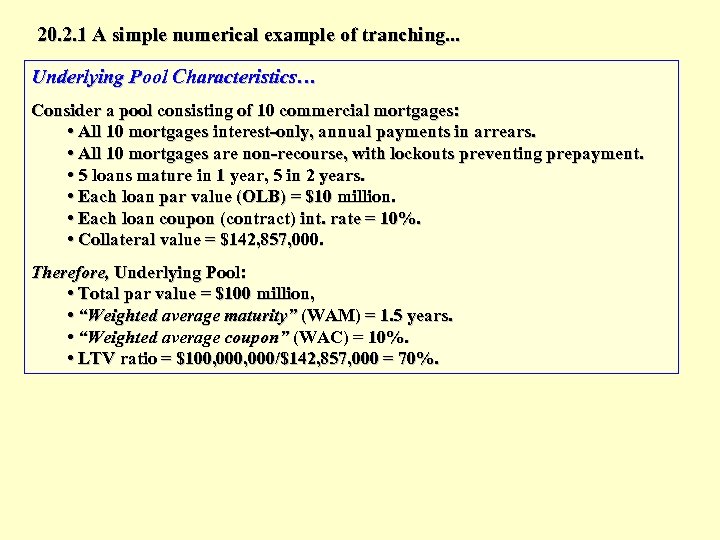
20. 2. 1 A simple numerical example of tranching. . . Underlying Pool Characteristics… Consider a pool consisting of 10 commercial mortgages: • All 10 mortgages interest-only, annual payments in arrears. • All 10 mortgages are non-recourse, with lockouts preventing prepayment. • 5 loans mature in 1 year, 5 in 2 years. • Each loan par value (OLB) = $10 million. • Each loan coupon (contract) int. rate = 10%. • Collateral value = $142, 857, 000. Therefore, Underlying Pool: • Total par value = $100 million, • “Weighted average maturity” (WAM) = 1. 5 years. • “Weighted average coupon” (WAC) = 10%. • LTV ratio = $100, 000/$142, 857, 000 = 70%.

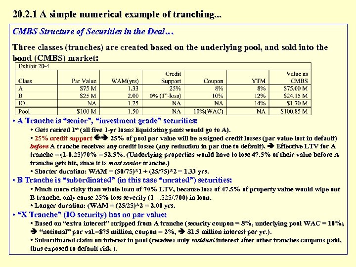
20. 2. 1 A simple numerical example of tranching. . . CMBS Structure of Securities in the Deal… Three classes (tranches) are created based on the underlying pool, and sold into the bond (CMBS) market: • A Tranche is “senior”, “investment grade” securities: • Gets retired 1 st (all five 1 -yr loans liquidating pmts would go to A). • 25% credit support 25% of pool par value will be assigned credit losses (par value lost in default) before A tranche receives any credit losses (any reduction in par due to default). Effective LTV for A tranche = (1 -0. 25)70% = 52. 5%. (Underlying properties would have to lose 47. 5% of their value before A tranche gets hit, since it is most senior tranche. ) • Shorter duration: WAM = (50/75)*1 + (25/75)*2 = 1. 33 yrs. • B Tranche is “subordinated” (in this case “unrated”) securities: • Much more risky than whole loan of 70% LTV, because loss of 47. 5% of property value would wipe out B tranche, only cause 25% loss severity (1 -. 525/. 700) in loan. • Longer duration: (WAM = (25/25)*2 = 2. 00 yrs. • “X Tranche” (IO security) has no par value: • Based on “extra interest” stripped from A tranche (security coupon = 8%, underlying pool WAC = 10%; “notional” par val. =$75 million, coupon = 2%, $1. 5 million interest per yr. ). • Subordinated claim on interest in pool (receives only residual interest after other tranches coupons paid, thus exposed to default risk ).

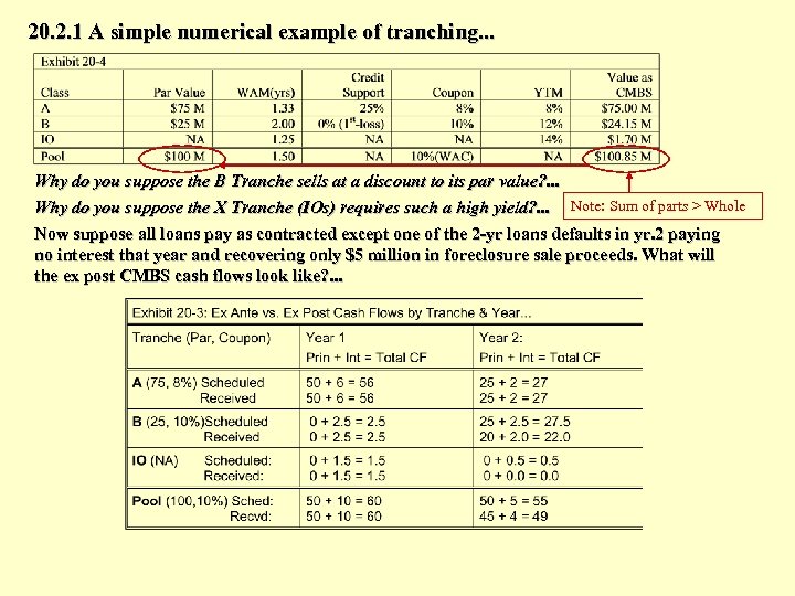
20. 2. 1 A simple numerical example of tranching. . . Why do you suppose the B Tranche sells at a discount to its par value? . . . Why do you suppose the X Tranche (IOs) requires such a high yield? . . . Note: Sum of parts > Whole Now suppose all loans pay as contracted except one of the 2 -yr loans defaults in yr. 2 paying no interest that year and recovering only $5 million in foreclosure sale proceeds. What will the ex post CMBS cash flows look like? . . .

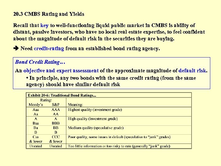
20. 3 CMBS Rating and Yields Recall that key to well-functioning liquid public market in CMBS is ability of distant, passive investors, who have no local real estate expertise, to feel confident about the magnitude of default risk in the securities they are buying. Need credit-rating from an established bond rating agency. Bond Credit Rating… An objective and expert assessment of the approximate magnitude of default risk. • In principle, any two bonds with the same credit rating (from the same agency) should have similar default risk

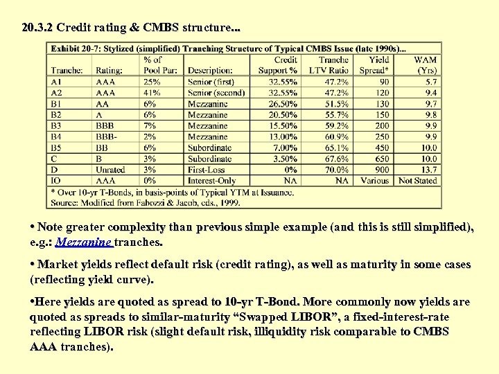
20. 3. 2 Credit rating & CMBS structure. . . • Note greater complexity than previous simple example (and this is still simplified), e. g. : Mezzanine tranches. • Market yields reflect default risk (credit rating), as well as maturity in some cases (reflecting yield curve). • Here yields are quoted as spread to 10 -yr T-Bond. More commonly now yields are quoted as spreads to similar-maturity “Swapped LIBOR”, a fixed-interest-rate reflecting LIBOR risk (slight default risk, illiquidity risk comparable to CMBS AAA tranches).

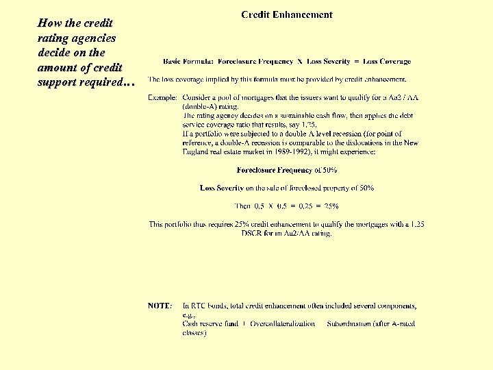
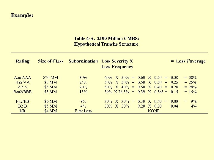
• The credit-rating a CMBS tranche receives is a function of the nature and risk of the underlying mortgage pool as well as of the amount of credit support in the tranche. • e. g. , a mortgage pool consisting of loans that have relatively low and homogeneous LTV ratios will not need as much credit support for a given credit-rating. Therefore, a larger proportion of the securities issued from such a pool can have higher credit-ratings, which means lower yields, thereby enabling the overall CMBS issue to obtain a higher average price and greater total proceeds. • Holding the quality of the underlying mortgage pool constant, greater credit support will result in a higher rating for a given tranche. • For example, an underlying pool with good quality information and a 60% LTV ratio might require only 20% credit support for a AAA rating, enabling 80% of the issue’s total par value to go into senior tranches. • In contrast, a more heterogeneous pool with an average LTV ratio of 75% and some questionable appraisals might require 45% credit support for a AA rating, allowing only 55% of the pool to be sold at a high-priced senior level. • It is the job of the bond-rating agency to figure out how much credit support is required for a given credit-rating for each tranche in a CMBS issue. The CMBS issuer works with the rating agency in an iterative security design process to develop the structure of the issue. • For example, if the rating agency requires 35% credit support for a AAA rating and 30% for a AA rating, it is then up to the CMBS issuer to decide whether to structure the senior tranche as a AAA-rated tranche containing 65% of the pool, or as a AA-rated tranche containing 70% of the pool.

Bond buyers draw a sharp distinction between investmentgrade and high-yield Source: JPMorgan Fleming

How the credit rating agencies decide on the amount of credit support required…

Example:

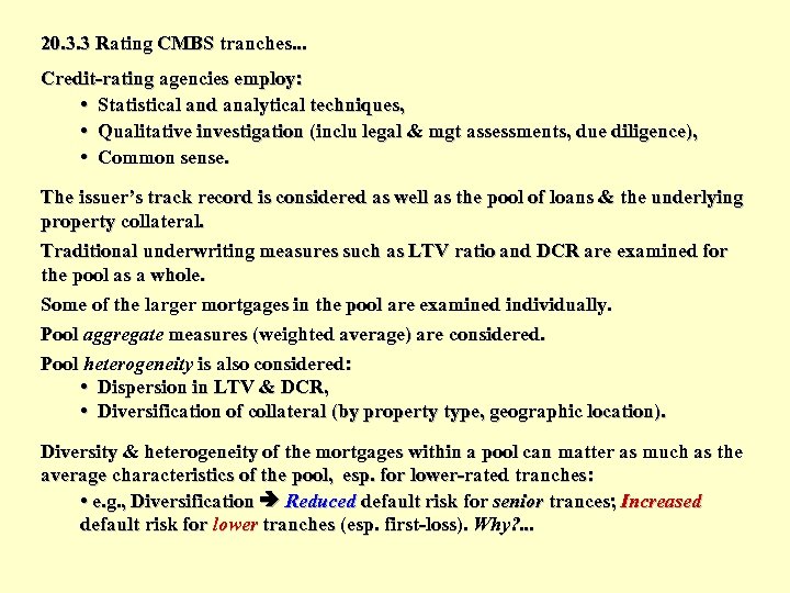
20. 3. 3 Rating CMBS tranches. . . Credit-rating agencies employ: • Statistical and analytical techniques, • Qualitative investigation (inclu legal & mgt assessments, due diligence), • Common sense. The issuer’s track record is considered as well as the pool of loans & the underlying property collateral. Traditional underwriting measures such as LTV ratio and DCR are examined for the pool as a whole. Some of the larger mortgages in the pool are examined individually. Pool aggregate measures (weighted average) are considered. Pool heterogeneity is also considered: • Dispersion in LTV & DCR, • Diversification of collateral (by property type, geographic location). Diversity & heterogeneity of the mortgages within a pool can matter as much as the average characteristics of the pool, esp. for lower-rated tranches: • e. g. , Diversification Reduced default risk for senior trances; Increased default risk for lower tranches (esp. first-loss). Why? . . .

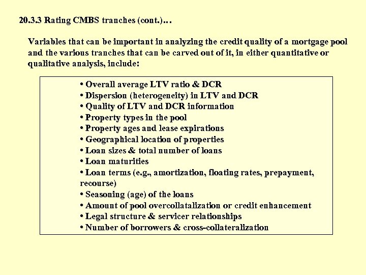
20. 3. 3 Rating CMBS tranches (cont. )… Variables that can be important in analyzing the credit quality of a mortgage pool and the various tranches that can be carved out of it, in either quantitative or qualitative analysis, include: • Overall average LTV ratio & DCR • Dispersion (heterogeneity) in LTV and DCR • Quality of LTV and DCR information • Property types in the pool • Property ages and lease expirations • Geographical location of properties • Loan sizes & total number of loans • Loan maturities • Loan terms (e. g. , amortization, floating rates, prepayment, recourse) • Seasoning (age) of the loans • Amount of pool overcollatalization or credit enhancement • Legal structure & servicer relationships • Number of borrowers & cross-collateralization

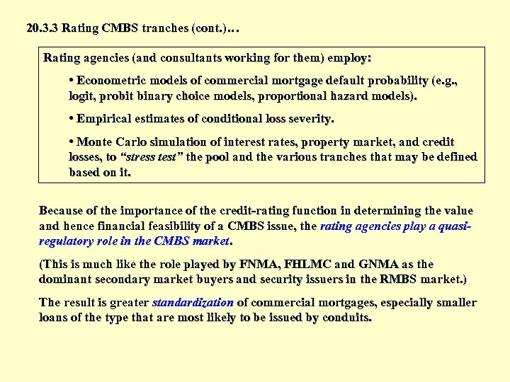
20. 3. 3 Rating CMBS tranches (cont. )… Rating agencies (and consultants working for them) employ: • Econometric models of commercial mortgage default probability (e. g. , logit, probit binary choice models, proportional hazard models). • Empirical estimates of conditional loss severity. • Monte Carlo simulation of interest rates, property market, and credit losses, to “stress test” the pool and the various tranches that may be defined based on it. Because of the importance of the credit-rating function in determining the value and hence financial feasibility of a CMBS issue, the rating agencies play a quasiregulatory role in the CMBS market. (This is much like the role played by FNMA, FHLMC and GNMA as the dominant secondary market buyers and security issuers in the RMBS market. ) The result is greater standardization of commercial mortgages, especially smaller loans of the type that are most likely to be issued by conduits.

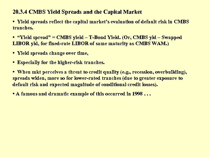
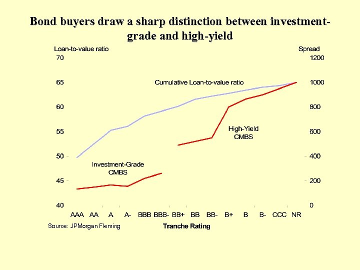
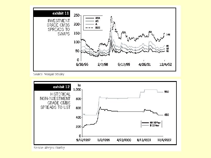
20. 3. 4 CMBS Yield Spreads and the Capital Market • Yield spreads reflect the capital market’s evaluation of default risk in CMBS tranches. • “Yield spread” = CMBS yield – T-Bond Yield. (Or, CMBS yld – Swapped LIBOR yld, for fixed-rate LIBOR of same maturity as CMBS WAM. ) • Yield spreads change over time, • Especially for the higher-risk tranches. • When mkt perceives a threat to credit quality (e. g. , recession, overbuilding), spreads widen, more so for lower-rated tranches (due to greater exposure to default risk and expected magnitude of conditional credit losses). • A famous and dramatic example of this occurred in 1998. . .

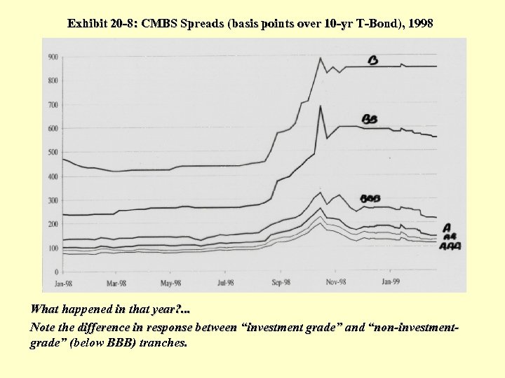
Exhibit 20 -8: CMBS Spreads (basis points over 10 -yr T-Bond), 1998 What happened in that year? . . . Note the difference in response between “investment grade” and “non-investmentgrade” (below BBB) tranches.

The 1998 crisis may have been a “textbook example” of how the public capital markets can help to effectively regulate the flow of capital to the real estate sector: the “negative feedback loop” in the real estate system described in Chapter 2… • The jump in yields for lower-rated CMBS depicted in Exhibit 20 -8 effectively eliminated the market for new issues of CMBS by the fall of 1998: • Commercial property investors and developers who had been planning to borrow money using the CMBS market as an indirect source of funds (e. g. , through conduit mortgages), would have to face interest rates so high, and/or LTV ratio limits so low, that the financial feasibility of their investments and developments would be called into question. • (REIT share prices also tumbled in 1998, temporarily also eliminating new REIT equity issues as a source of capital for real estate. ) • As a result, the flow of capital reaching the real estate sector was cut back. • This reduction in capital flow put some breaks on new construction, directly or indirectly resulting in less new space supply coming into the system than otherwise would have been the case at that time.

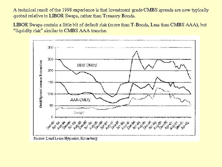
A technical result of the 1998 experience is that investment grade CMBS spreads are now typically quoted relative to LIBOR Swaps, rather than Treasury Bonds. LIBOR Swaps contain a little bit of default risk (more than T-Bonds, Less than CMBS AAA), but “liquidity risk” similar to CMBS AAA tranche.

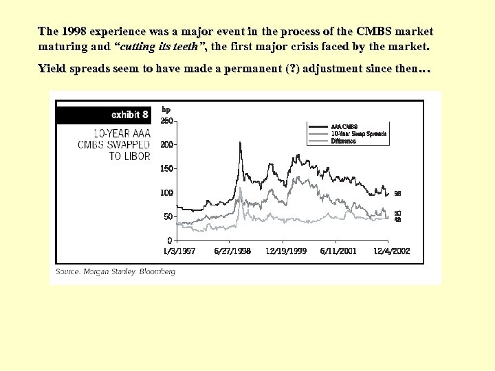
The 1998 experience was a major event in the process of the CMBS market maturing and “cutting its teeth”, the first major crisis faced by the market. Yield spreads seem to have made a permanent (? ) adjustment since then…

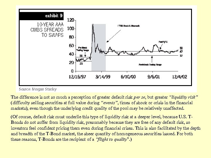
The difference is not so much a perception of greater default risk per se, but greater “liquidity risk” (difficulty selling securities at full value during “events”, times of shock or crisis in the financial markets), even though the underlying credit quality of the pool may be relatively unaffected. (Of course, default risk must underlie this type of liquidity risk at a deeper level, because U. S. TBonds do not suffer from liquidity risk, presumably because they are free of any default risk, so investors feel confident pricing them even during financial crises. This is also facilitated by the depth and breadth of the T-Bond market, the sheer quantity of homogeneous securities issued. For both these reasons, T-Bonds are the recipient of a “flight to quality”. )

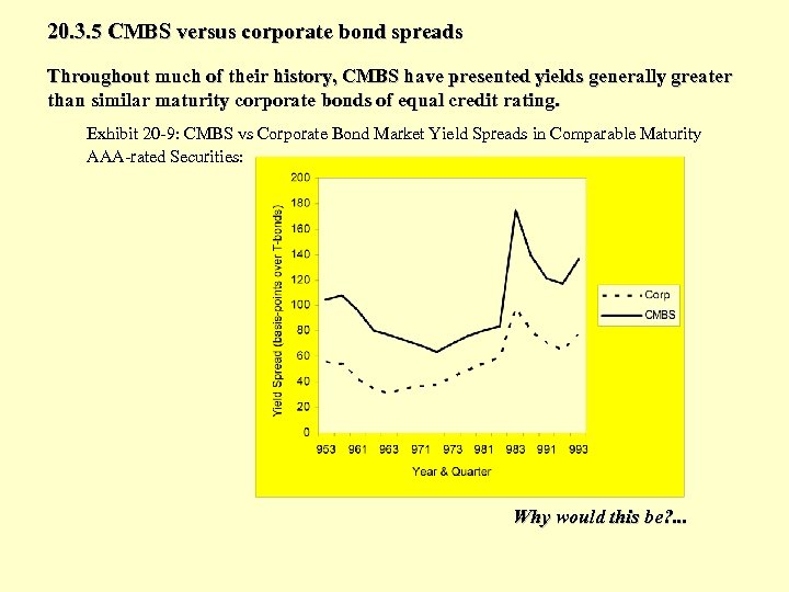
20. 3. 5 CMBS versus corporate bond spreads Throughout much of their history, CMBS have presented yields generally greater than similar maturity corporate bonds of equal credit rating. Exhibit 20 -9: CMBS vs Corporate Bond Market Yield Spreads in Comparable Maturity AAA-rated Securities: Why would this be? . . .

20. 3. 5 CMBS versus corporate bond spreads CMBS are “different animals” compared to corporate bonds: 1. Prepayment Risk: Most U. S. commercial mortgs have “prepayment protection”, but some do not (or it is imperfect, or goes away). Some CMBS pools contain mortgages that are more like callable corporate bonds, resulting in a yield premium to reflect the prepayment risk faced by the investor. Such a yield premium would affect spreads for all tranches, but especially for senior tranches, given the typical principal payback priority structure. 2. Agency and Extension Risk: In the event of default in CMBS pools, a conflict of interest tends to exist between investors in senior versus junior tranches. The former want immediate foreclosure, while the latter tend to prefer a workout and extension of loan term. The authority to decide whether to foreclose or exercise forebearance is vested in the “special servicer”, who is usually effectively controlled by the junior tranche holders (after all, they stand to lose or gain the most from how the default is handled). Foreclosure/workout decision cannot be expected to be handled optimally from the senior tranche holders’ perspective. Higher yield in the senior tranches. No such conflict of interest exists in typical corporate bonds because there is only one class of investor. 3. Credit Information Quality and Going-concern Risk & Liquidity Implications: Bonds backed by large publicly-traded corporations have available more on-going information relevant to the credit risk of the borrower. Also, the public corporation is a single going-concern that typically knows it will need to return to the bond market again, probably regularly in the near and longterm future. It therefore must carefully consider its reputation in the bond market, and this makes it less likely to default on its bonds. Rating agencies and investors are more “in the dark” about the credit risk of the typical CMBS issue than they are with the typical corporate bond. This concern is especially relevant for the lower-rated tranches.

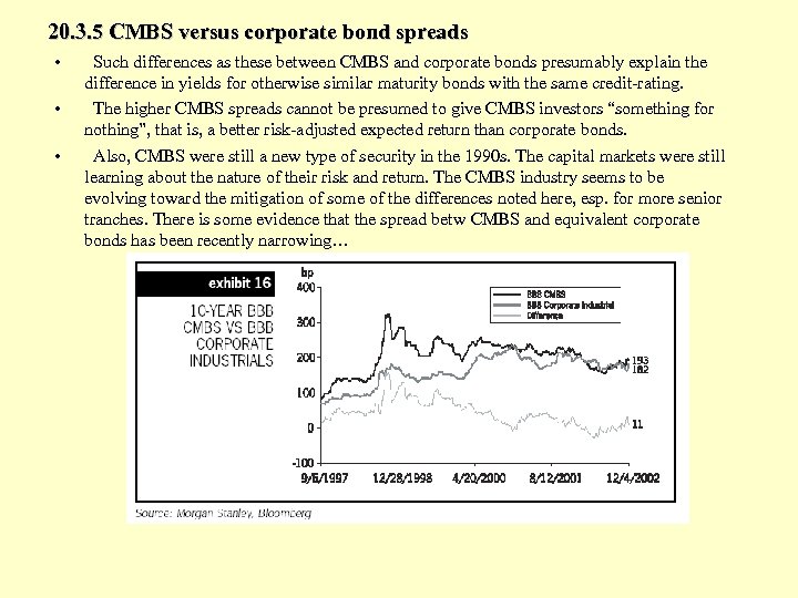
20. 3. 5 CMBS versus corporate bond spreads • • • Such differences as these between CMBS and corporate bonds presumably explain the difference in yields for otherwise similar maturity bonds with the same credit-rating. The higher CMBS spreads cannot be presumed to give CMBS investors “something for nothing”, that is, a better risk-adjusted expected return than corporate bonds. Also, CMBS were still a new type of security in the 1990 s. The capital markets were still learning about the nature of their risk and return. The CMBS industry seems to be evolving toward the mitigation of some of the differences noted here, esp. for more senior tranches. There is some evidence that the spread betw CMBS and equivalent corporate bonds has been recently narrowing…

Ch. 20 CMBS Summary; • CMBS have unique investment characteristics (relatively little prepayment risk, relatively high yields) that appeal to important classes of investors, thereby increasing the capital available to real estate, and improving the efficiency of the functioning of the capital market for investors. • Variety in the risk and return attributes of the securities carved out of a mortgage pool allow different tranches to appeal to different types of investors. • The CMBS market is another example of how investor heterogeneity drives the investment industry. • Typically, the investment-grade tranches that make up the bulk of a typical CMBS issue find ready buyers in the form of conservative institutions such as pension funds, life insurance companies, and bond mutual funds. • The market for the more risky speculative and junk tranches is much thinner. • Major buyers and holders of the lower tranches are aggressive investors willing to take on risk for high expected returns, and who typically have specialized knowledge and expertise regarding commercial property risk. • Such investors have included the investment banks and conduits issuing the CMBS, the “special servicers” who are charged with taking over defaulted loans in the pool to attempt “workouts” with the borrowers, and specialized mortgage REITs.

Aside… Prepayment Protection in Commercial Mortgages Due to their history as a prime investment for institutions interested in “maturity matching” (such as LICs), commercial mortgages have traditionally incorporated much more “prepayment protection” (aka “call protection”) than residential mortgages. Four major types of prepayment protection, listed in order from most to least protective: 1. “Hard Lockout”: Forbids prepayment prior to loan maturity. 2. “Defeasance”: Borrower must purchase T-Bond strips to provide lender with same cash flows as mortgage for remaining life of mortgage. * (T-Bond collateral substitutes property collateral, resulting in lower default risk, hence increased value for lender. ) 3. “Yield Maintenance Provision”: Borrower pays a “make whole” penalty to lender. Typical requirement would be penalty equal to PV of difference between loan interest and current T-Bond interest (for bond of maturity equal to remaining maturity on loan), with the PV calculated based on T-Bond yield as the discount rate. 4. “Fixed Percentage Penalty Points”: Borrower pays stated percentage over the OLB on the loan. 5. Note: Many loans mix two or more of the above. (e. g. , lockout period followed by points penalty that declines with further age of loan. )

Chapter 17 Section 17. 3: The Refinancing Decision If a loan has a prepayment option, the borrower can choose to pay the loan off early to take advantage of favorable interest rate movements, “refinancing” the old loan with a new, cheaper loan. This refinancing decision can be evaluated by comparing two loans, the existing (“old”) loan and a “new” loan that would replace it. Traditionally, this comparison is made using the classical DCF methodology. In this section, we will first present this traditional approach, then we will explore something important that is left out of the traditional picture, namely, the prepayment option value in the old loan.

17. 3: The Refinancing Decision Compare two loans. NPV (of refinancing, to borrower) = Value of Old Loan Liability – Value of New Loan Exactly Replacing Old Loan This NPV is the evaluation (decision) framework. OCC (disc. rate, “r”) = Eff. int. rate in current loan market (“mkt yield”). Basic principles (“apples vs apples”): 1) Compare over same time horizon; 2) Compare over the same debt amount. Overview of solution steps: 1) Compute NPV of incremental CFs of having New Loan instead of Old Loan (keeping in mind the “apples vs apples” principles). 2) Subtract from this the transaction cost of obtaining the New Loan (e. g. , title insurance, appraisal fees, etc). This gives the NPV of refinancing, except for: 3) Subtract the value of the refinancing option in the Old Loan, which you are giving up when you refinance. (This is the “prepayment option”, the call option on a bond. ) Steps (1) & (2) are all that is presented in typical R. E. finance textbooks. Unfortunately, the option value can often swamp the NPV result from the first two steps.

17. 3. 1 The traditional refinancing calculation Let: PV(CFOLD) = DCF based present value of Old Loan. PV(CFNEW) = DCF based present value of New (replacement) Loan. “PV()” DCF procedure, CFOLD = Remaining cash flows in the old loan. CFNEW = Future cash flow stream in the new loan (after its initial disbursement to the borrower). “Apples-vs-apples” comparison • Both loans evaluated over the same time horizon, and for the same loan amount. • Both loans must be evaluated using the current opportunity cost of capital as the discount rate. NPV(of refinancing for borrower) = PV(CFOLD) – PV(CFNEW), less any transaction costs the borrower faces in the refinancing deal

17. 3. 1 The traditional refinancing calculation This procedure is equivalent to calculating the net incremental difference in cash flows each period under the new loan compared to the old, and summing the present values of these periodic savings to the borrower. Using the same discount rate (the current opportunity cost of capital), the difference in the present values of the cash flows equals the present value of the differences in the cash flows*: PV(CFOLD)-PV(CFNEW) = PV(CFOLD-CFNEW). Normally, the savings from refinancing will occur in the regular monthly payments, while the last cash flow in the analysis time horizon may involve an incremental cost to the borrower, as the new loan may at that time have a larger outstanding balance than the old loan would have had.

17. 3. 1 The traditional refinancing calculation To implement this DCF procedure in practice, specify: • Common time horizon = Expected time until the old loan would be likely to be paid off in the absence of refinancing: • This is at the latest is the maturity date of the old loan. This may be earlier than the maturity of the replacement loan, under which case the replacement loan must be evaluated with expected cash flows corresponding to such early prepayment of the replacement loan. • Amount of Debt = What is necessary for borrower to exactly pay off the old loan: • . If new loan has a disbursement discount, then the contractual principal borrowed on the new loan must exceed the old loan OLB plus prepayment penalty on the old loan (such that refinancing transaction is zero net cash flow except for transaction costs). • OCC (discount rate) = The current mkt yield on the new loan, computed over the common time horizon: • If the new loan has any disbursement discounts, or if the new loan has a prepayment penalty and the common time horizon is prior to the new loan’s maturity, then this discount rate will, of course, exceed the contract interest rate in the new loan.

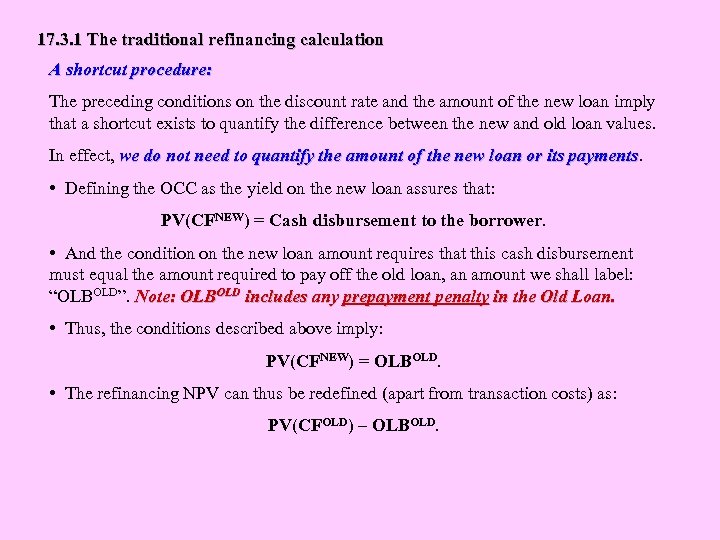
17. 3. 1 The traditional refinancing calculation A shortcut procedure: The preceding conditions on the discount rate and the amount of the new loan imply that a shortcut exists to quantify the difference between the new and old loan values. In effect, we do not need to quantify the amount of the new loan or its payments • Defining the OCC as the yield on the new loan assures that: PV(CFNEW) = Cash disbursement to the borrower. • And the condition on the new loan amount requires that this cash disbursement must equal the amount required to pay off the old loan, an amount we shall label: “OLBOLD”. Note: OLBOLD includes any prepayment penalty in the Old Loan. • Thus, the conditions described above imply: PV(CFNEW) = OLBOLD. • The refinancing NPV can thus be redefined (apart from transaction costs) as: PV(CFOLD) – OLBOLD.

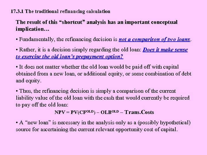
17. 3. 1 The traditional refinancing calculation The result of this “shortcut” analysis has an important conceptual implication… • Fundamentally, the refinancing decision is not a comparison of two loans. • Rather, it is a decision simply regarding the old loan: Does it make sense to exercise the old loan’s prepayment option? • It does not matter whether the old loan would be paid off with capital obtained from a new loan, or additional equity, or some combination of debt and equity. • Thus, the refinancing decision is simply a comparison of the current liability value of the old loan with the cash that would currently be required to pay off the old loan: NPV = PV(CFOLD) – OLBOLD – Trans. Costs • A “new loan” is necessary in the analysis only as a (possibly hypothetical) source for ascertaining the current relevant opportunity cost of capital.

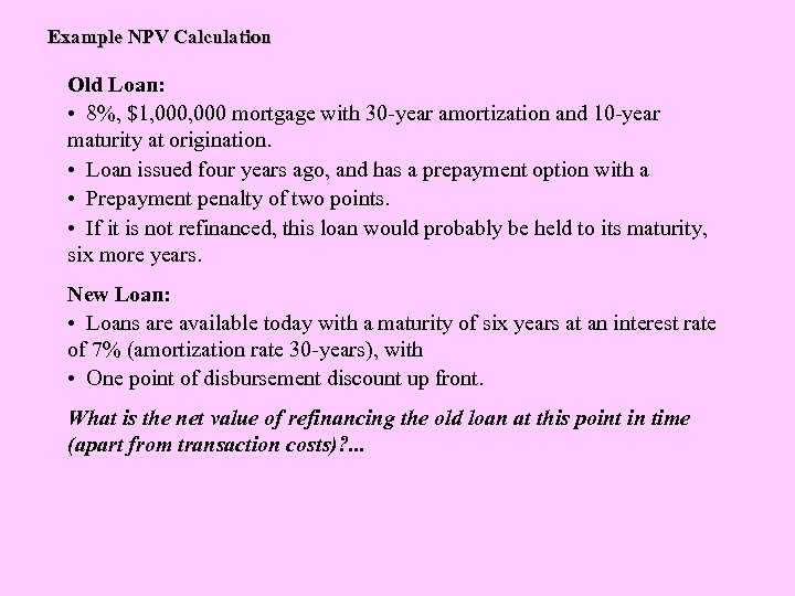
Example NPV Calculation Old Loan: • 8%, $1, 000 mortgage with 30 -year amortization and 10 -year maturity at origination. • Loan issued four years ago, and has a prepayment option with a • Prepayment penalty of two points. • If it is not refinanced, this loan would probably be held to its maturity, six more years. New Loan: • Loans are available today with a maturity of six years at an interest rate of 7% (amortization rate 30 -years), with • One point of disbursement discount up front. What is the net value of refinancing the old loan at this point in time (apart from transaction costs)? . . .

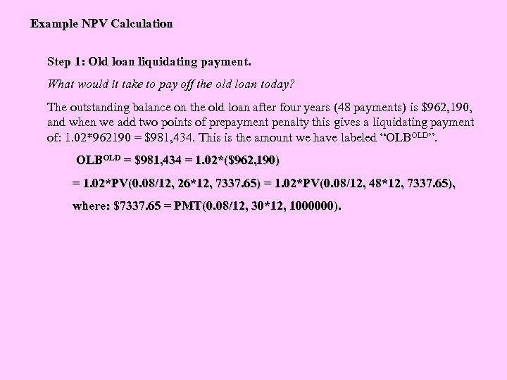
Example NPV Calculation Step 1: Old loan liquidating payment. What would it take to pay off the old loan today? The outstanding balance on the old loan after four years (48 payments) is $962, 190, and when we add two points of prepayment penalty this gives a liquidating payment of: 1. 02*962190 = $981, 434. This is the amount we have labeled “OLBOLD”. OLBOLD = $981, 434 = 1. 02*($962, 190) = 1. 02*PV(0. 08/12, 26*12, 7337. 65) = 1. 02*PV(0. 08/12, 48*12, 7337. 65), where: $7337. 65 = PMT(0. 08/12, 30*12, 1000000).

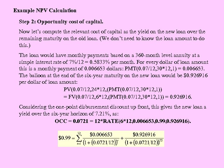
Example NPV Calculation Step 2: Opportunity cost of capital. Now let’s compute the relevant cost of capital as the yield on the new loan over the remaining maturity on the old loan. (We don’t need to know the loan amount to do this. ) The loan would have monthly payments based on a 360 -month level annuity at a simple interest rate of 7%/12 = 0. 5833% per month. For every dollar of loan amount this is a monthly payment of 0. 006653 dollars: PMT(0. 07/12, 30*12, 1) = 0. 006653. The balloon at the end of the six-year maturity on the new loan would be $0. 926916 per dollar of loan amount: PV(0. 07/12, 24*12, (PMT(0. 07/12, 30*12, 1)) = FV(0. 07/12, 6*12, (PMT(0. 07/12, 30*12, 1)) = 0. 926916. Considering the one-point disbursement discount up front, this gives the new loan a yield over the six-year horizon of 7. 21%, as: OCC = 0. 0721 = 12*RATE(6*12, 0. 006653, 0. 99, 0. 926916).

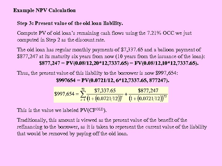
Example NPV Calculation Step 3: Present value of the old loan liability. Compute PV of old loan’s remaining cash flows using the 7. 21% OCC we just computed in Step 2 as the discount rate. The old loan has regular monthly payments of $7, 337. 65 and a balloon payment of $877, 247 at its maturity six years from now (10 years from the issuance of the loan): $877, 247 = PV(0. 08/12, 20*12, 7337. 65) = FV(0. 08/12, 10*12, 7337. 65). Thus, the present value of this liability to the borrower is now $997, 654: $997654 = PV(0. 0721/12, 6*12, 7337. 65, 877247). This is the value we labeled PV(CFOLD). Traditionally, this amount is viewed as the present value of the benefit of the refinancing to the borrower, as it is taken to represent the current value of the liability that would be removed by paying off the old loan.

Example NPV Calculation Step 4: Compute the NPV(of refinancing to the borrower), before considering transaction costs = PV(benefit) computed in Step 3 – Liquidating payment computed in Step 1: NPV = $997, 654 - $981, 434 = $16, 220. This is the value of PV(CFOLD)-OLBOLD, including the prepayment penalty in OLBOLD. According to the traditional analysis performed above, our example loan should be prepaid, as long as the transaction costs involved in obtaining the necessary capital are less than $16, 220. e. g. , if transaction costs = $10, 000, then the NPV of paying off the old loan would be $16, 220 - $10, 000 = $6, 220. Transaction costs typically include third-party fees, such as appraisal and title insurance costs that might not be included in the loan origination fee, or investment banker fees (in the case of equity capital). In addition, the borrower should consider their own costs involved in searching for replacement capital.

17. 3. 2 What is left out of the traditional calculation: Prepayment Option Value That the prepayment option has a positive value to the borrower can be seen in the previous calculations. We have determined that by exercising this option today the borrower could increase the market value of their net wealth by $6, 220, even after transaction costs. The prepayment option is worth at least this much. But in paying off the old loan, the borrower extinguishes this prepayment option. An option no longer exists after it is exercised. The loss of this option is therefore a cost to the borrower if they prepay the old loan. How much is this option worth?

Prepayment Option Value: A Simplified Example… In the previous example, the interest rate on the Old Loan was 8%, and the current interest rate (applicable to a New Loan) was 7%. But what will interest rates be in the future? . . . Suppose the probability for interest rates 1 year from now are: • 5% with 50% probability, • 9% with 50% probability. Use the same procedure as before to calculate the NPV of refinancing, as of next year, under each of the two possible future interest rate scenarios…

Prepayment Option Value: A Simplified Example… Suppose we believe the following subjective probability distribution describes what interest rates (on the new loan) will be like in one year: 5% with 50% chance; 9% with 50% chance. Now recalculate Steps 1 -4 NPV under each of these scenarios, one year from now (5 years gone by on the old loan, 5 more years to go in the holding horizon). Using the same procedures as indicated before, we get the following expected NPVs (after subtracting $10, 000 transaction costs) as of one year from now, under each interest rate scenario: NPV 1 = +$82, 448, if interest rates are 5%; NPV 1 = -$75, 078, if interest rates are 9%. (Obviously it does not make sense for the borrower to refinance an 8% loan with a new 9% loan. )

Prepayment Option Value: A Simplified Example… Thus, if the 9% interest rate scenario transpires, you would not refinance, but simply keep the old loan. In that case you would face a NPV=0 effect (from doing nothing). This reflects the fact that options are rights without obligation. As a result, as of today the expected NPV next year due to the refinancing option in the old loan is: E 0[refin 1] = (50%)*(82448) + (50%)*(0) = $41, 224. What is the present value of this expected value one year from now? Option values are risky, so they should be discounted at a high discount rate reflecting a large risk premium in the opportunity cost of capital. Suppose we require a 30% per annum return on holding the option. Then the PV today of the refinancing option in the old loan is: PV[refin 1] = 41224 / 1. 30 = +$31, 711. Thus, under the above assumptions, the refinancing option in the old loan is worth $31, 711. This value would be given up if we refinance today. In return, we would obtain the +$6, 220 NPV from the exercise of the refinancing option today (previously calculated). Thus, including the prepayment option value in the refinancing calculation reveals that it does not make sense to refinance today: NPV[refin 0] = NPV 0 - PV[refin 1] = 6220 - 31711 = -$25, 491

Prepayment Option Value: A Simplified Example… This same result can also be obtained by properly including the prepayment option value in the valuation of the old loan. The prepayment option value is positive to the borrower, but negative to the lender. Labeling “C(Prepay)” as the market value of the prepayment option, and “D(Old)” as the market value of the old loan, we have: D(Old) = PV(CFOLD) – C(Prepay) (1) The market value based NPV of old loan prepayment, from the borrower’s perspective, is therefore: NPV(Prepay) = D(Old) – OLBOLD – TC (2) where “TC” is the borrower’s transaction costs in the deal. Equation (2) simply says that when the market value of the existing loan exceeds the cash that would be required to pay off that loan (including the transaction costs), then refinancing will have a positive impact on the borrower’s net wealth. As the market value of the old loan already incorporates the value of the prepayment option (which reflects the possible value of waiting to prepay the old loan later), paying off the old loan will be currently optimal for the borrower whenever equation (2) is positive.

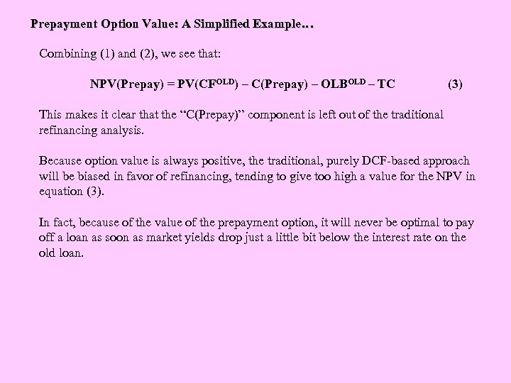
Prepayment Option Value: A Simplified Example… Combining (1) and (2), we see that: NPV(Prepay) = PV(CFOLD) – C(Prepay) – OLBOLD – TC (3) This makes it clear that the “C(Prepay)” component is left out of the traditional refinancing analysis. Because option value is always positive, the traditional, purely DCF-based approach will be biased in favor of refinancing, tending to give too high a value for the NPV in equation (3). In fact, because of the value of the prepayment option, it will never be optimal to pay off a loan as soon as market yields drop just a little bit below the interest rate on the old loan.