01343ae933ec289fd2e61463b4da6aad.ppt
- Количество слайдов: 90
Chapter 2 The Basics of Supply and Demand
Introduction l What are supply and demand? l What is the market mechanism? l What are the effects of changes in market equilibrium? l What are elasticities of supply and demand? © 2005 Pearson Education, Inc. Chapter 2 2

Topics to Be Discussed l How do short-run and long-run elasticities differ? l How do we understand predict the effects of changing market conditions? l What are the effects of government intervention – price controls? © 2005 Pearson Education, Inc. Chapter 2 3
Supply and Demand l Supply and demand analysis can: 1. Help us understand predict how world economic conditions affect market price and production 2. Analyze the impact of government price controls, minimum wages, price supports, and production incentives on the economy 3. Determine how taxes, subsidies, tariffs and import quotas affect consumers and producers © 2005 Pearson Education, Inc. Chapter 2 4

Supply and Demand l The Supply Curve m. The relationship between the quantity of a good that producers are willing to sell and the price of the good. m. Measures quantity on the x-axis and price on the y-axis © 2005 Pearson Education, Inc. Chapter 2 5
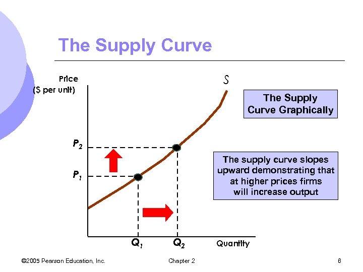
The Supply Curve S Price ($ per unit) The Supply Curve Graphically P 2 The supply curve slopes upward demonstrating that at higher prices firms will increase output P 1 Q 1 © 2005 Pearson Education, Inc. Q 2 Chapter 2 Quantity 6

The Supply Curve l Change in Quantity Supplied m. Movement along the curve caused by a change in price l Change in Supply m. Shift of the curve caused by a change in something other than price l Change © 2005 Pearson Education, Inc. in costs of production Chapter 2 7
Change in Supply l Other Variables Affecting Supply m. Costs of Production l Labor l Capital l Raw Materials m. Lower costs of production allow a firm to produce more at each price and vice versa © 2005 Pearson Education, Inc. Chapter 2 8
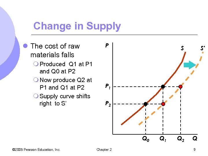
Change in Supply l The cost of raw materials falls m Produced Q 1 at P 1 and Q 0 at P 2 m Now produce Q 2 at P 1 and Q 1 at P 2 m Supply curve shifts right to S’ P S P 1 P 2 Q 0 © 2005 Pearson Education, Inc. S’ Chapter 2 Q 1 Q 2 Q 9
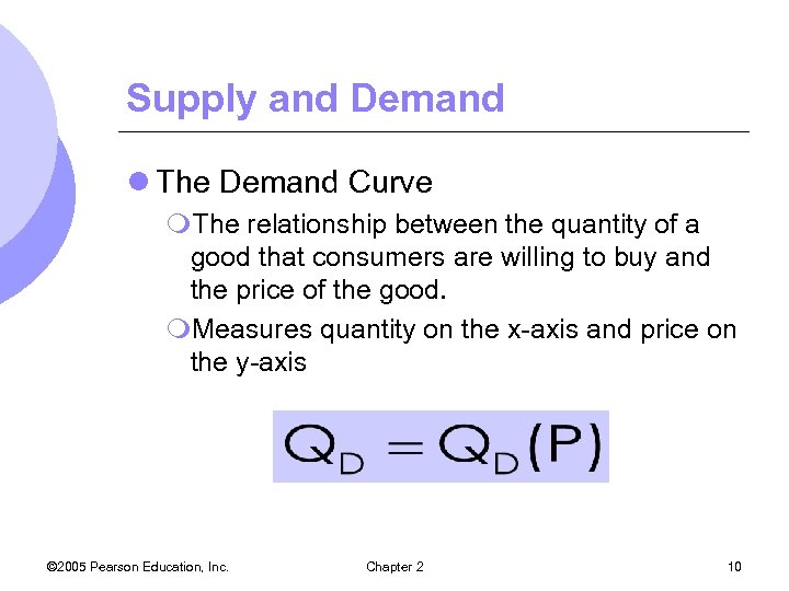
Supply and Demand l The Demand Curve m. The relationship between the quantity of a good that consumers are willing to buy and the price of the good. m. Measures quantity on the x-axis and price on the y-axis © 2005 Pearson Education, Inc. Chapter 2 10

The Demand Curve Price ($ per unit) The demand curve slopes downward demonstrating that consumers are willing to buy more at a lower price as the product becomes relatively cheaper. P 2 P 1 D Q 1 © 2005 Pearson Education, Inc. Q 2 Chapter 2 Quantity 11
The Demand Curve l Changes in quantity demanded m. Movements along the demand curve caused by a change in price. l Changes in demand m. A shift of the entire demand curve caused by something other than price. l Income l Preferences © 2005 Pearson Education, Inc. Chapter 2 12
Change in Demand l Other Variables Affecting Demand m. Income l Increases in income allow consumers to purchase more at all prices m. Consumer Tastes m. Price of Related Goods l Substitutes l Complements © 2005 Pearson Education, Inc. Chapter 2 13
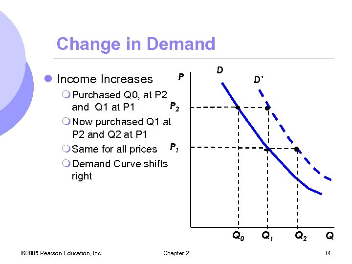
Change in Demand l Income Increases P D D’ m Purchased Q 0, at P 2 and Q 1 at P 1 m Now purchased Q 1 at P 2 and Q 2 at P 1 m Same for all prices P 1 m Demand Curve shifts right Q 0 © 2005 Pearson Education, Inc. Chapter 2 Q 1 Q 2 Q 14
The Market Mechanism l The market mechanism is the tendency in a free market for price to change until the market clears l Markets clear when quantity demanded equals quantity supplied at the prevailing price l Market Clearing price – price at which markets clear © 2005 Pearson Education, Inc. Chapter 2 15
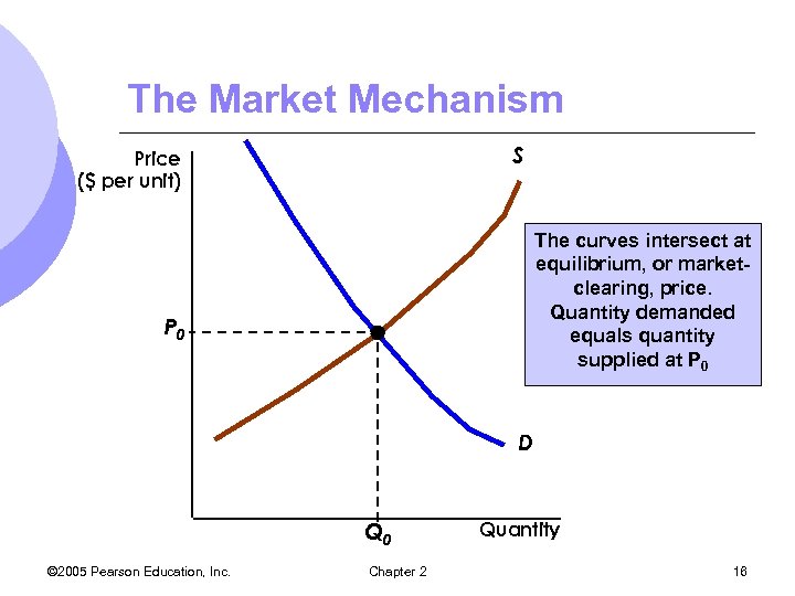
The Market Mechanism S Price ($ per unit) The curves intersect at equilibrium, or marketclearing, price. Quantity demanded equals quantity supplied at P 0 D Q 0 © 2005 Pearson Education, Inc. Chapter 2 Quantity 16
The Market Mechanism l In equilibrium m. There is no shortage or excess demand m. There is no surplus or excess supply m. Quantity supplied equals quantity demanded m. Anyone who wished to buy at the current price can and all producers who wish to sell at that price can © 2005 Pearson Education, Inc. Chapter 2 17
Market Surplus l The market price is above equilibrium m. There is excess supply - surplus m. Downward pressure on price m. Quantity demanded increases and quantity supplied decreases m. The market adjusts until new equilibrium is reached © 2005 Pearson Education, Inc. Chapter 2 18
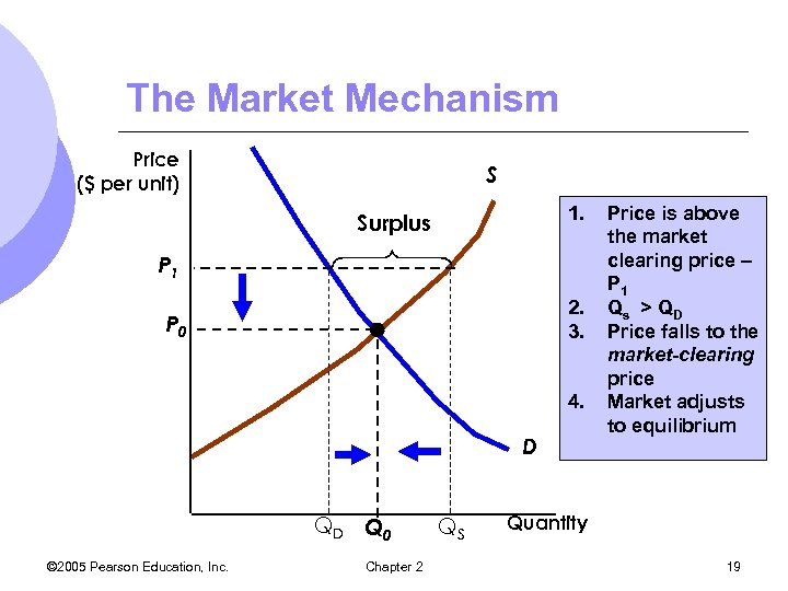
The Market Mechanism Price ($ per unit) S 1. Surplus P 1 2. 3. P 0 4. D QD Q 0 © 2005 Pearson Education, Inc. Chapter 2 QS Price is above the market clearing price – P 1 Qs > Q D Price falls to the market-clearing price Market adjusts to equilibrium Quantity 19
The Market Mechanism l The market price is below equilibrium: m. There is a excess demand - shortage m. Upward pressure on prices m. Quantity demanded decreases and quantity supplied increases m. The market adjusts until the new equilibrium is reached. © 2005 Pearson Education, Inc. Chapter 2 20
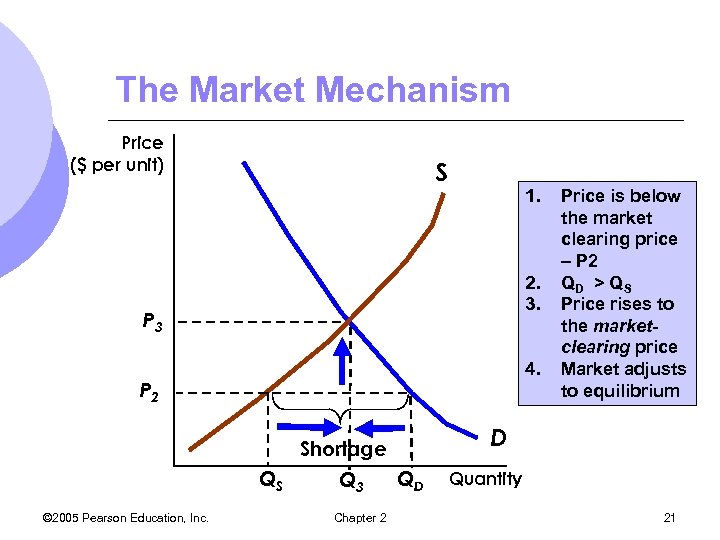
The Market Mechanism Price ($ per unit) S 1. 2. 3. P 3 4. P 2 D Shortage QS © 2005 Pearson Education, Inc. Q 3 Chapter 2 Price is below the market clearing price – P 2 QD > Q S Price rises to the marketclearing price Market adjusts to equilibrium QD Quantity 21
The Market Mechanism l Supply and demand interact to determine the market-clearing price. l When not in equilibrium, the market will adjust to alleviate a shortage or surplus and return the market to equilibrium. l Markets must be competitive for the mechanism to be efficient. © 2005 Pearson Education, Inc. Chapter 2 22

Changes In Market Equilibrium l Equilibrium prices are determined by the relative level of supply and demand. l Changes in supply and/or demand will change in the equilibrium price and/or quantity in a free market. © 2005 Pearson Education, Inc. Chapter 2 23
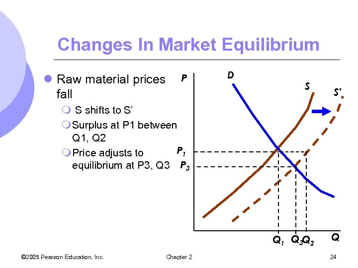
Changes In Market Equilibrium l Raw material prices fall P D S S’ m S shifts to S’ m Surplus at P 1 between Q 1, Q 2 P 1 m Price adjusts to equilibrium at P 3, Q 3 P 3 Q 1 Q 3 Q 2 © 2005 Pearson Education, Inc. Chapter 2 Q 24
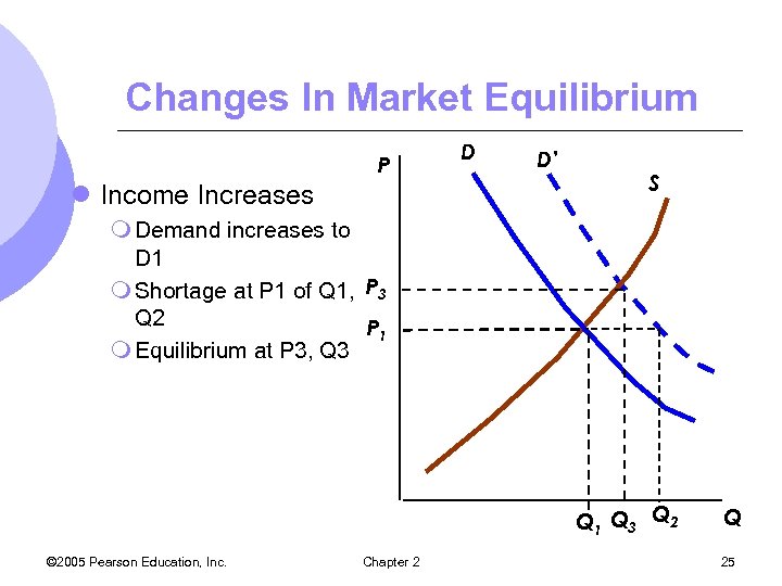
Changes In Market Equilibrium P l Income Increases D D’ S m Demand increases to D 1 m Shortage at P 1 of Q 1, P 3 Q 2 P 1 m Equilibrium at P 3, Q 3 Q 1 Q 3 Q 2 © 2005 Pearson Education, Inc. Chapter 2 Q 25

Changes In Market Equilibrium l Income Increases & raw material prices fall m Quantity increases m If the increase in D is greater than the increase in S price also increases P D D’ S S’ P 2 P 1 Q 1 © 2005 Pearson Education, Inc. Chapter 2 Q 26
Shifts in Supply and Demand l When supply and demand change simultaneously, the impact on the equilibrium price and quantity is determined by: 1. The relative size and direction of the change 2. The shape of the supply and demand models © 2005 Pearson Education, Inc. Chapter 2 27

The Price of a College Education l The real price of a college education rose 55 percent from 1970 to 2002. l Increases in costs of modern classrooms and wages increased costs of production – decrease in supply l Due to a larger percentage of high school graduates attending college, demand increased © 2005 Pearson Education, Inc. Chapter 2 28
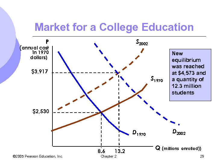
Market for a College Education S 2002 P (annual cost in 1970 dollars) $3, 917 S 1970 New equilibrium was reached at $4, 573 and a quantity of 12. 3 million students $2, 530 D 1970 © 2005 Pearson Education, Inc. 8. 6 13. 2 Chapter 2 D 2002 Q (millions enrolled)) 29
The Long-Run Behavior of Natural Resource Prices m. Consumption of copper has increased about a hundred fold from 1880 through 2002. m. The long term real price for copper has remained relatively constant. m. Increased demand as world economy grew m. Decreased production costs increased supply © 2005 Pearson Education, Inc. Chapter 2 30
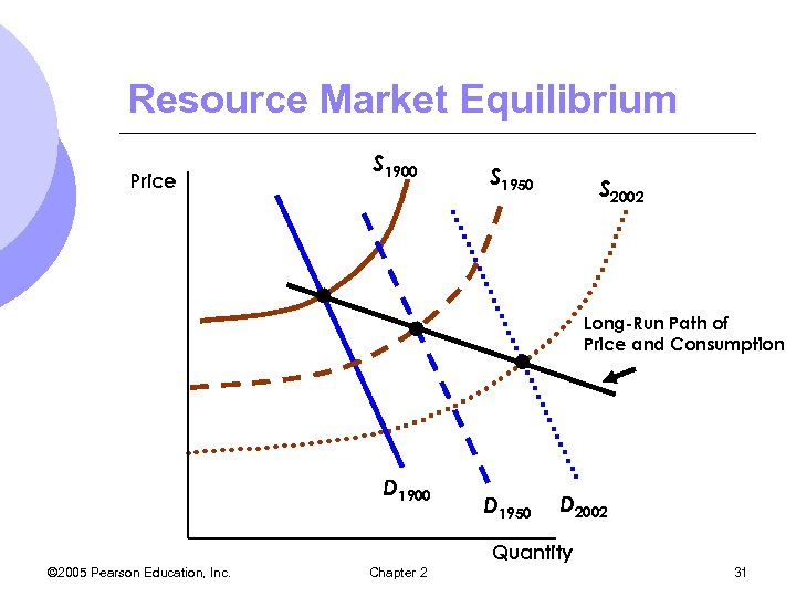
Resource Market Equilibrium Price S 1900 S 1950 S 2002 Long-Run Path of Price and Consumption D 1900 D 1950 D 2002 Quantity © 2005 Pearson Education, Inc. Chapter 2 31
Resource Market l Conclusion m. Decreases in the costs of production have increased the supply by more than enough to offset the increase in demand. © 2005 Pearson Education, Inc. Chapter 2 32

Elasticities of Supply and Demand l Not only are we concerned with what direction price and quantity will move when the market changes, but we are concerned about how much they change. l Elasticity gives a way to measure by how much a variable will change with the change in another variable. l Specifically, it gives the percentage change in one variable resulting from a one percent change in another. © 2005 Pearson Education, Inc. Chapter 2 33
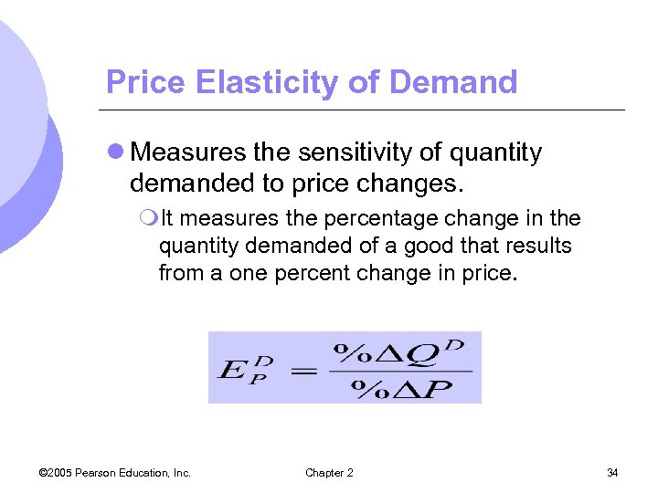
Price Elasticity of Demand l Measures the sensitivity of quantity demanded to price changes. m. It measures the percentage change in the quantity demanded of a good that results from a one percent change in price. © 2005 Pearson Education, Inc. Chapter 2 34
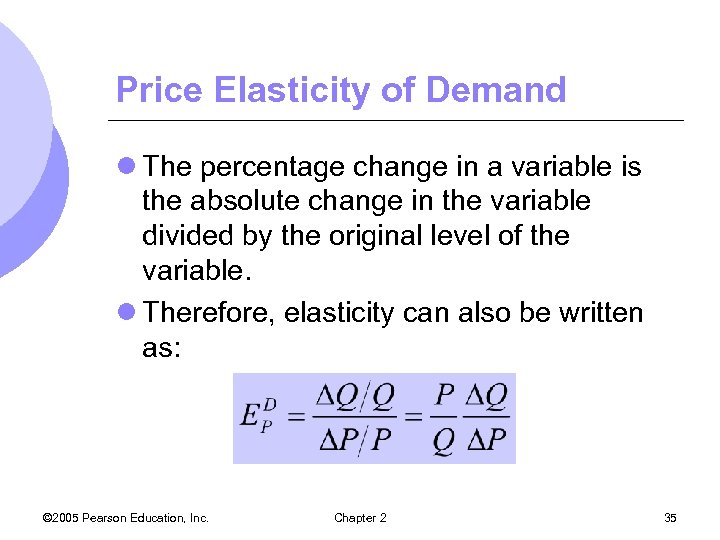
Price Elasticity of Demand l The percentage change in a variable is the absolute change in the variable divided by the original level of the variable. l Therefore, elasticity can also be written as: © 2005 Pearson Education, Inc. Chapter 2 35
Price Elasticity of Demand l Usually a negative number m. As price increases, quantity decreases m. As price decreases, quantity increases l When EP > 1, the good is price elastic m% Q > % P l When EP < 1, the good is price inelastic m% Q < % P © 2005 Pearson Education, Inc. Chapter 2 36
Price Elasticity of Demand l The primary determinant of price elasticity of demand is the availability of substitutes. m. Many substitutes demand is price elastic l Can easily move to another good with price increases m. Few substitutes demand is price inelastic © 2005 Pearson Education, Inc. Chapter 2 37

Price Elasticity of Demand l Looking at a linear demand curve, as we move along the curve Q/ P will change l Price elasticity of demand must therefore be measured at a particular point on the demand curve l Elasticity will change along the demand curve in a particular way © 2005 Pearson Education, Inc. Chapter 2 38

Price Elasticity of Demand l Given a linear demand curve m. Elasticity depends on slope and on the values of P and Q m. The top portion of demand curve is elastic l Price is high and quantity small m. The bottom portion of demand curve is inelastic l Price © 2005 Pearson Education, Inc. is low and quantity high Chapter 2 39

Price Elasticity of Demand Price 4 EP = - Demand Curve Q = 8 – 2 P Elastic Ep = -1 2 Inelastic 4 © 2005 Pearson Education, Inc. 8 Chapter 2 Q Ep = 0 40
Price Elasticity of Demand l The steeper the demand curve becomes, the more inelastic the good. l The flatter the demand curve becomes, the more elastic the good l Two extreme cases of demand curves m. Completely inelastic demand – vertical m. Infinitely elastic demand - horizontal © 2005 Pearson Education, Inc. Chapter 2 41
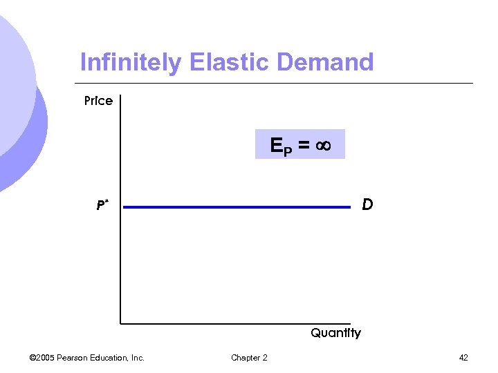
Infinitely Elastic Demand Price EP = D P* Quantity © 2005 Pearson Education, Inc. Chapter 2 42
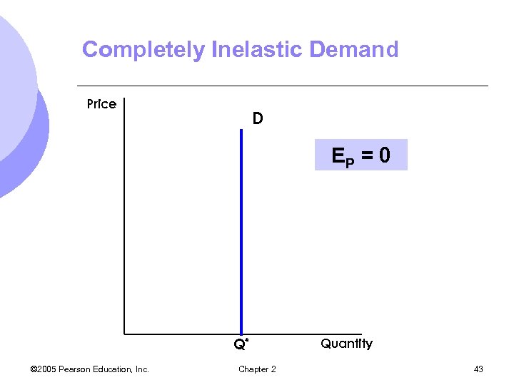
Completely Inelastic Demand Price D EP = 0 Q* © 2005 Pearson Education, Inc. Chapter 2 Quantity 43
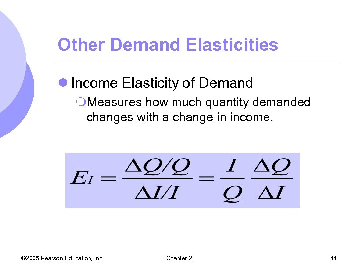
Other Demand Elasticities l Income Elasticity of Demand m. Measures how much quantity demanded changes with a change in income. © 2005 Pearson Education, Inc. Chapter 2 44
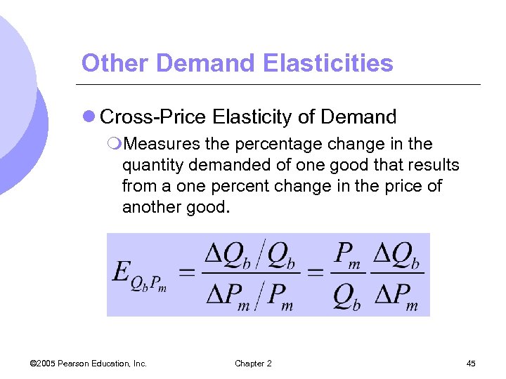
Other Demand Elasticities l Cross-Price Elasticity of Demand m. Measures the percentage change in the quantity demanded of one good that results from a one percent change in the price of another good. © 2005 Pearson Education, Inc. Chapter 2 45
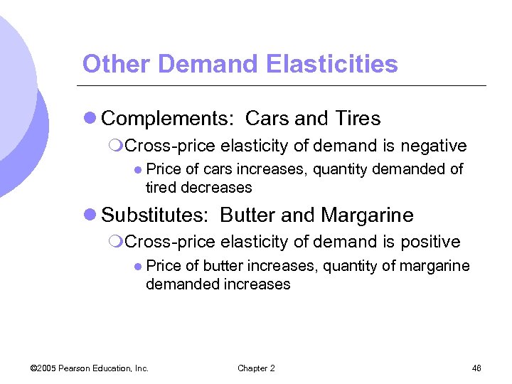
Other Demand Elasticities l Complements: Cars and Tires m. Cross-price elasticity of demand is negative l Price of cars increases, quantity demanded of tired decreases l Substitutes: Butter and Margarine m. Cross-price elasticity of demand is positive l Price of butter increases, quantity of margarine demanded increases © 2005 Pearson Education, Inc. Chapter 2 46
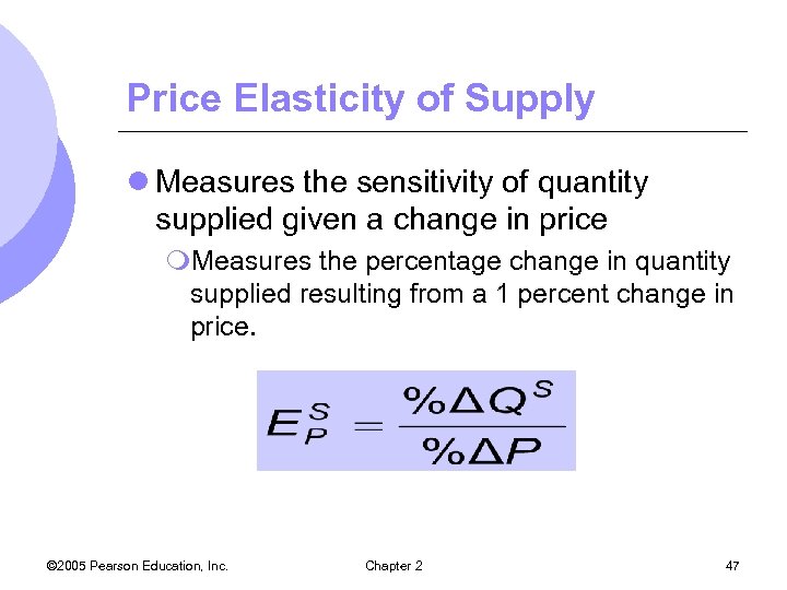
Price Elasticity of Supply l Measures the sensitivity of quantity supplied given a change in price m. Measures the percentage change in quantity supplied resulting from a 1 percent change in price. © 2005 Pearson Education, Inc. Chapter 2 47

Point v. Arc Elasticities l Point elasticity of demand m. Price elasticity of demand at a particular point on the demand curve l Arc elasticity of demand m. Price elasticity of demand calculated over a range of prices © 2005 Pearson Education, Inc. Chapter 2 48
Elasticity: An Application l During 1980’s and 1990’s, market for wheat went through changes that had great implications for American farmers and US agricultural policy l Using the supply and demand curves for wheat, we can analyze what occurred in this market © 2005 Pearson Education, Inc. Chapter 2 49
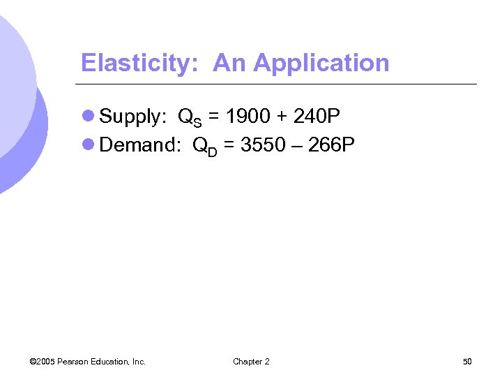
Elasticity: An Application l Supply: QS = 1900 + 240 P l Demand: QD = 3550 – 266 P © 2005 Pearson Education, Inc. Chapter 2 50
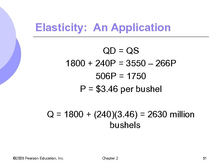
Elasticity: An Application QD = QS 1800 + 240 P = 3550 – 266 P 506 P = 1750 P = $3. 46 per bushel Q = 1800 + (240)(3. 46) = 2630 million bushels © 2005 Pearson Education, Inc. Chapter 2 51
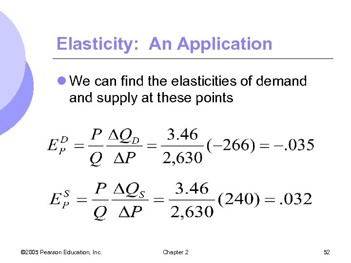
Elasticity: An Application l We can find the elasticities of demand supply at these points © 2005 Pearson Education, Inc. Chapter 2 52

Elasticity: An Application l Assume the price of wheat is $4. 00/bushel due to decrease in supply © 2005 Pearson Education, Inc. Chapter 2 53

Elasticity: An Application l In 2002, the supply and demand for wheat were: m. Supply: QS = 1439 + 267 P m. Demand: QD = 2809 – 226 P © 2005 Pearson Education, Inc. Chapter 2 54
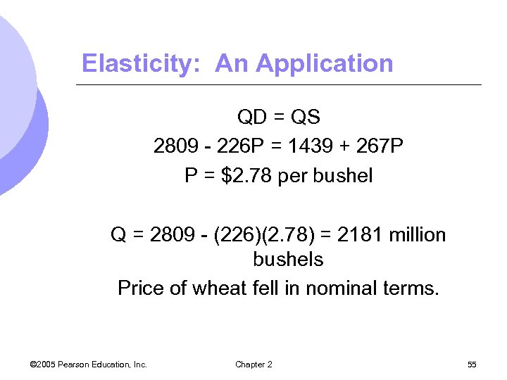
Elasticity: An Application QD = QS 2809 - 226 P = 1439 + 267 P P = $2. 78 per bushel Q = 2809 - (226)(2. 78) = 2181 million bushels Price of wheat fell in nominal terms. © 2005 Pearson Education, Inc. Chapter 2 55
Short-Run Versus Long-Run Elasticity l Price elasticity varies with the amount of time consumers have to respond to a price. l Short run demand supply curves often look very different from their longrun counterparts. © 2005 Pearson Education, Inc. Chapter 2 56
Short-Run Versus Long-Run Elasticity l Demand m. In general, demand is much more price elastic in the long run l Consumers take time to adjust consumption habits l Demand might be linked to another good that changes slowly l More substitutes are usually available in the long run © 2005 Pearson Education, Inc. Chapter 2 57
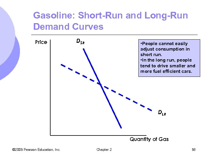
Gasoline: Short-Run and Long-Run Demand Curves Price DSR • People cannot easily adjust consumption in short run. • In the long run, people tend to drive smaller and more fuel efficient cars. DLR Quantity of Gas © 2005 Pearson Education, Inc. Chapter 2 58

Short-Run Versus Long-Run Elasticity l Demand Durability m. For some durable goods, demand is more elastic in the short run m. If goods are durable, then when price increases, consumers choose to hold on to the good instead of replacing it so its quantity demanded fall sharply. m. But in long run, older durable goods will have to be replaced © 2005 Pearson Education, Inc. Chapter 2 59
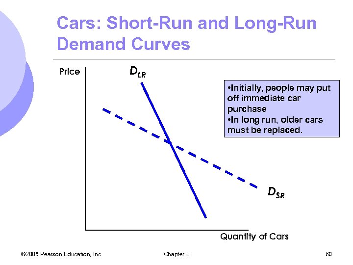
Cars: Short-Run and Long-Run Demand Curves Price DLR • Initially, people may put off immediate car purchase • In long run, older cars must be replaced. DSR Quantity of Cars © 2005 Pearson Education, Inc. Chapter 2 60
Short-Run Versus Long-Run Elasticity l Income elasticity also varies with the amount of time consumers have to respond to an income change. m. For most goods and services, income elasticity is larger in the long run m. When income changes, it takes time to adjust spending © 2005 Pearson Education, Inc. Chapter 2 61
Short-Run Versus Long-Run Elasticity l Income elasticity of durable goods m. Income elasticity is less in the long-run than in the short-run. l Increases in income mean consumers will want to hold more cars. l Once older cars replaced, purchases will only to be to replace old cars. l Less purchases from income increase in long run than in short run © 2005 Pearson Education, Inc. Chapter 2 62
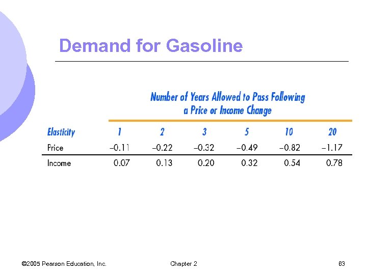
Demand for Gasoline © 2005 Pearson Education, Inc. Chapter 2 63
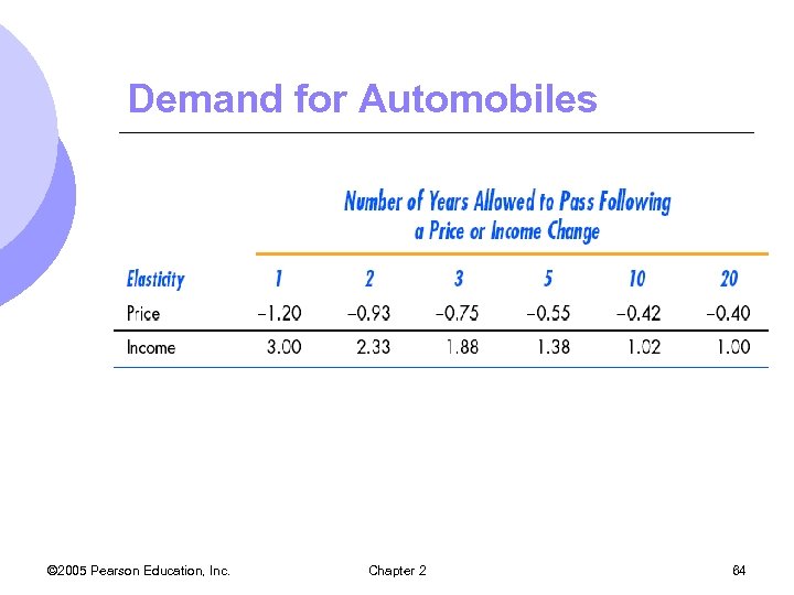
Demand for Automobiles © 2005 Pearson Education, Inc. Chapter 2 64
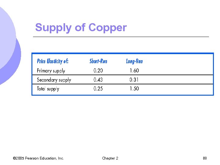
Short-Run Versus Long-Run Elasticity l Most goods and services: m. Long-run price elasticity of supply is greater than short-run price elasticity of supply. l Other Goods (durables, recyclables): m. Long-run price elasticity of supply is less than short-run price elasticity of supply © 2005 Pearson Education, Inc. Chapter 2 65
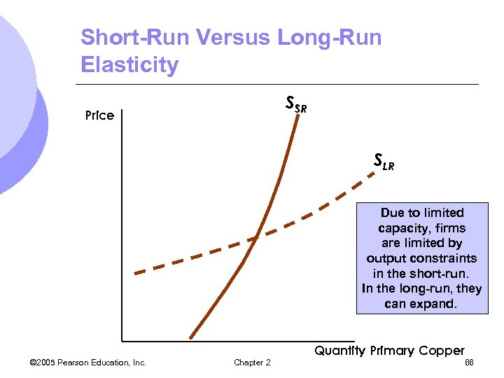
Short-Run Versus Long-Run Elasticity SSR Price SLR Due to limited capacity, firms are limited by output constraints in the short-run. In the long-run, they can expand. Quantity Primary Copper © 2005 Pearson Education, Inc. Chapter 2 66
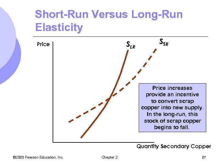
Short-Run Versus Long-Run Elasticity SLR Price SSR Price increases provide an incentive to convert scrap copper into new supply. In the long-run, this stock of scrap copper begins to fall. Quantity Secondary Copper © 2005 Pearson Education, Inc. Chapter 2 67
Supply of Copper © 2005 Pearson Education, Inc. Chapter 2 68

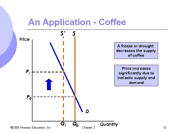
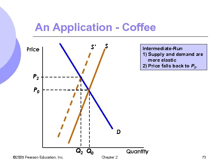
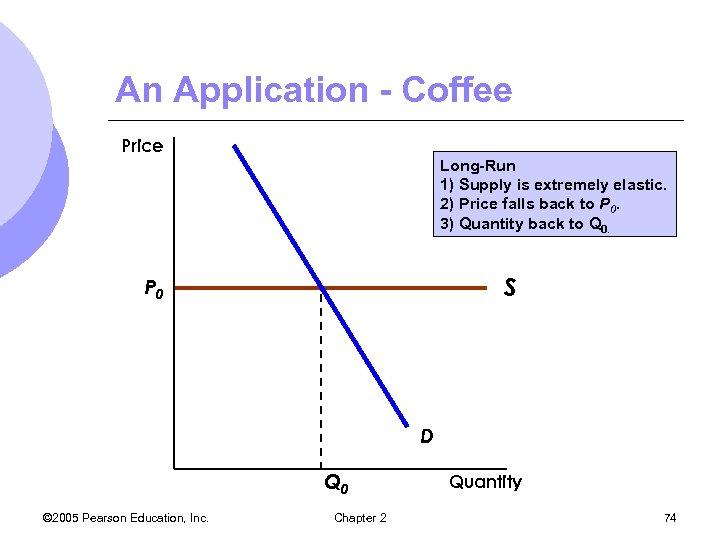
Short-Run v. Long-Run Elasticity – An Application l Why are coffee prices very volatile? m. Most of the world’s coffee produced in Brazil. m. Many changing weather conditions affect the crop of coffee, thereby affecting price m. Price following bad weather conditions is usually short-lived m. In long run, prices come back to original levels, all else equal © 2005 Pearson Education, Inc. Chapter 2 69

Price of Brazilian Coffee © 2005 Pearson Education, Inc. Chapter 2 70

Short-Run v. Long-Run Elasticity – An Application l Demand supply are more elastic in the long run l In short-run, supply is completely inelastic m. Weather may destroy part of the fixed supply, decreasing supply l Demand relatively inelastic as well l Price increases significantly © 2005 Pearson Education, Inc. Chapter 2 71
An Application - Coffee Price S’ S A freeze or drought decreases the supply of coffee Price increases significantly due to inelastic supply and demand P 1 P 0 D © 2005 Pearson Education, Inc. Q 1 Q 0 Chapter 2 Quantity 72
An Application - Coffee Price S’ S Intermediate-Run 1) Supply and demand are more elastic 2) Price falls back to P 2 P 0 D © 2005 Pearson Education, Inc. Q 2 Q 0 Quantity Chapter 2 73
An Application - Coffee Price Long-Run 1) Supply is extremely elastic. 2) Price falls back to P 0. 3) Quantity back to Q 0. S P 0 D Q 0 © 2005 Pearson Education, Inc. Chapter 2 Quantity 74

Predicting the Effects of Changing Market Conditions l Supply and demand analysis can be used to predict the effects of changing market conditions m. Linear demand supply must be fit to market data l Given equilibrium price and quantity along with elasticities of supply and demand, we can calculate the curves that fit the information l We can then calculate changes in the market © 2005 Pearson Education, Inc. Chapter 2 75
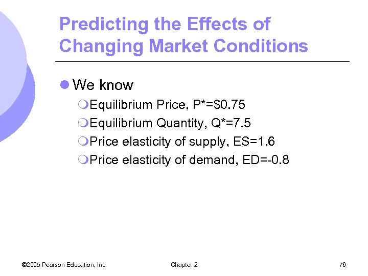
Predicting the Effects of Changing Market Conditions l We know m. Equilibrium Price, P*=$0. 75 m. Equilibrium Quantity, Q*=7. 5 m. Price elasticity of supply, ES=1. 6 m. Price elasticity of demand, ED=-0. 8 © 2005 Pearson Education, Inc. Chapter 2 76
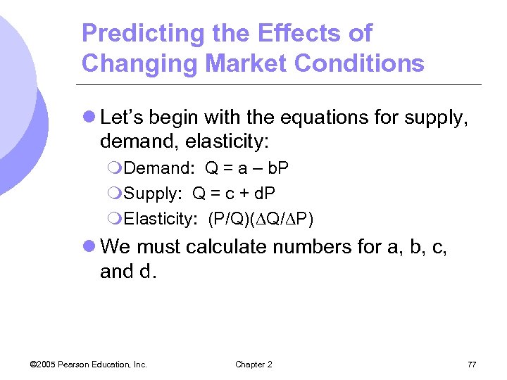
Predicting the Effects of Changing Market Conditions l Let’s begin with the equations for supply, demand, elasticity: m. Demand: Q = a – b. P m. Supply: Q = c + d. P m. Elasticity: (P/Q)( Q/ P) l We must calculate numbers for a, b, c, and d. © 2005 Pearson Education, Inc. Chapter 2 77
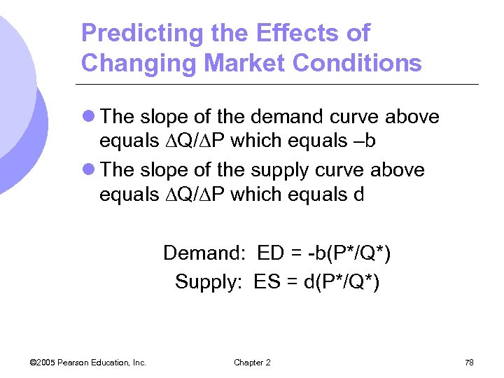
Predicting the Effects of Changing Market Conditions l The slope of the demand curve above equals Q/ P which equals –b l The slope of the supply curve above equals Q/ P which equals d Demand: ED = -b(P*/Q*) Supply: ES = d(P*/Q*) © 2005 Pearson Education, Inc. Chapter 2 78
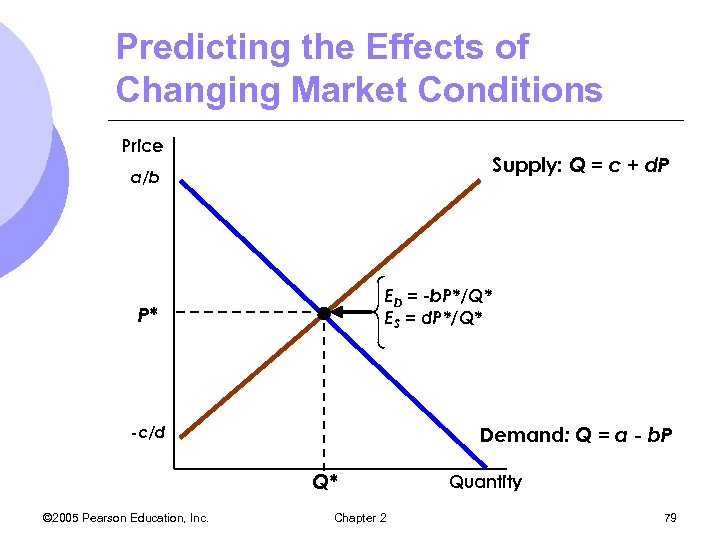
Predicting the Effects of Changing Market Conditions Price Supply: Q = c + d. P a/b ED = -b. P*/Q* ES = d. P*/Q* P* Demand: Q = a - b. P -c/d Q* © 2005 Pearson Education, Inc. Chapter 2 Quantity 79
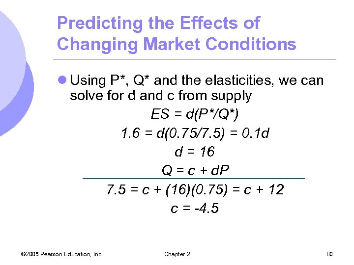
Predicting the Effects of Changing Market Conditions l Using P*, Q* and the elasticities, we can solve for d and c from supply ES = d(P*/Q*) 1. 6 = d(0. 75/7. 5) = 0. 1 d d = 16 Q = c + d. P 7. 5 = c + (16)(0. 75) = c + 12 c = -4. 5 © 2005 Pearson Education, Inc. Chapter 2 80
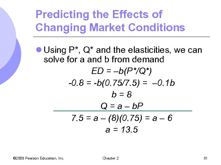
Predicting the Effects of Changing Market Conditions l Using P*, Q* and the elasticities, we can solve for a and b from demand ED = –b(P*/Q*) -0. 8 = -b(0. 75/7. 5) = – 0. 1 b b=8 Q = a – b. P 7. 5 = a – (8)(0. 75) = a – 6 a = 13. 5 © 2005 Pearson Education, Inc. Chapter 2 81
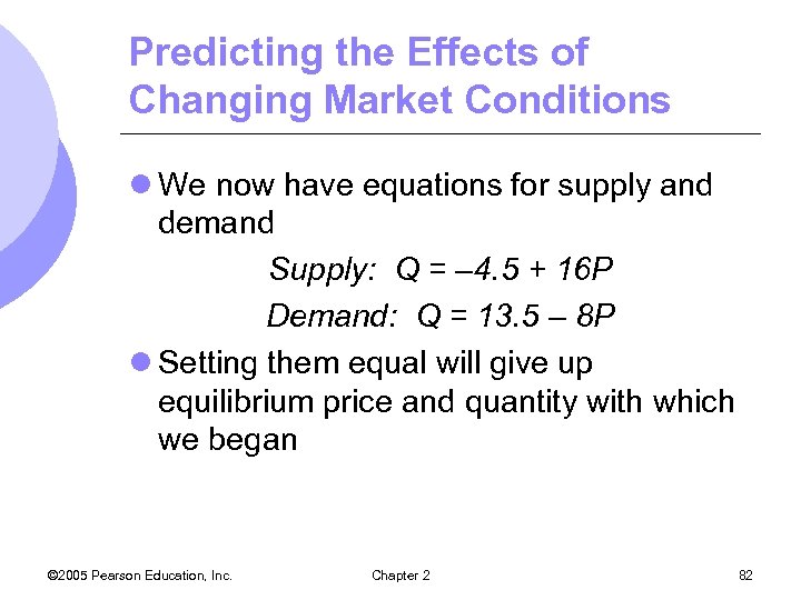
Predicting the Effects of Changing Market Conditions l We now have equations for supply and demand Supply: Q = – 4. 5 + 16 P Demand: Q = 13. 5 – 8 P l Setting them equal will give up equilibrium price and quantity with which we began © 2005 Pearson Education, Inc. Chapter 2 82
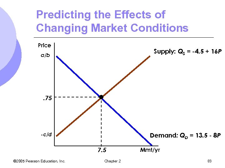
Predicting the Effects of Changing Market Conditions Price Supply: QS = -4. 5 + 16 P a/b . 75 Demand: QD = 13. 5 - 8 P -c/d 7. 5 © 2005 Pearson Education, Inc. Chapter 2 Mmt/yr 83
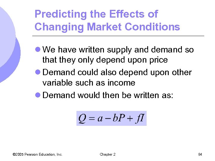
Predicting the Effects of Changing Market Conditions l We have written supply and demand so that they only depend upon price l Demand could also depend upon other variable such as income l Demand would then be written as: © 2005 Pearson Education, Inc. Chapter 2 84

Predicting the Effects of Changing Market Conditions l We know the following information regarding the copper industry: m. I = 1. 0 m. P* = 0. 75 m. Q* = 7. 5 mb = 8 m. Income elasticity: E I= 1. 3 © 2005 Pearson Education, Inc. Chapter 2 85
Predicting the Effects of Changing Market Conditions l Using the elasticity of income formula, we can solve for f EI = (I/Q)( Q/ I) 1. 3 = (1. 0/7. 5)(f) f = 9. 75 l Substituting back into demand equation gives a = 3. 75 © 2005 Pearson Education, Inc. Chapter 2 86
Effects of Price Controls l Markets are rarely free of government intervention m. Imposed taxes and granted subsidies m. Price controls l Price controls usually hold the price above or below the equilibrium price m. Excess demand – shortage m. Excess supply - surplus © 2005 Pearson Education, Inc. Chapter 2 87
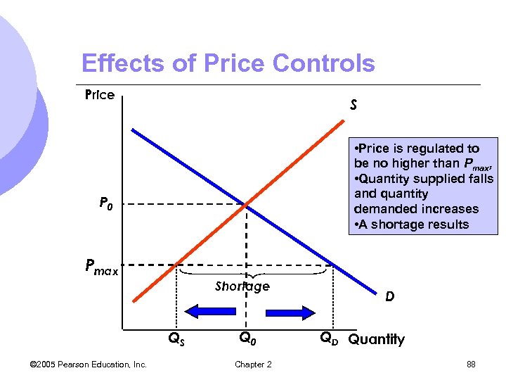
Effects of Price Controls Price S • Price is regulated to be no higher than Pmax, • Quantity supplied falls and quantity demanded increases • A shortage results P 0 Pmax Shortage QS © 2005 Pearson Education, Inc. Q 0 Chapter 2 D QD Quantity 88
Effects of Price Controls l Excess demand sometimes takes the form of queues m. Lines at gas stations during 1974 shortage l Sometimes get curtailments and supply rationing m. Natural gas shortage of the mid ’ 70’s l Producers typically lose, but some consumers gain. Some consumers lose. © 2005 Pearson Education, Inc. Chapter 2 89
Price Controls and Natural Gas Shortages l In 1954, the federal government began regulating the wellhead price of natural gas. l In 1962, the ceiling prices that were imposed became binding and shortages resulted. l Price controls created an excess demand of 7 trillion cubic feet. © 2005 Pearson Education, Inc. Chapter 2 90
01343ae933ec289fd2e61463b4da6aad.ppt