Chapter 2 Technology Costs and Market Structure 1

Chapter 2 Technology, Costs and Market Structure 1

Introduction • Industries have very different structures – numbers and size distributions of firms • ready-to-eat breakfast cereals: high concentration Top 4 firms account for about 80% of sales • Games and toys (not including video games): The largest 4 firms accounts for 35% to 45% • How best to measure market structure – summary measure (p 55, Figure 2 -1) – concentration curve is possible – preference is for a single number – concentration ratio or Herfindahl-Hirschman index (HHI) 2

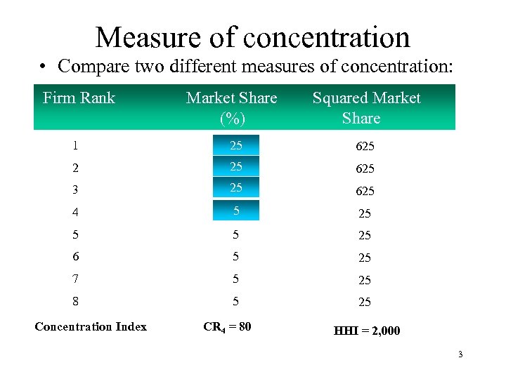Measure of concentration • Compare two different measures of concentration: Firm Rank Market Share (%) Squared Market Share 1 25 625 2 25 625 3 25 625 4 5 25 5 5 25 6 5 25 7 5 25 8 5 25 Concentration Index CR 4 = 80 HHI = 2, 000 3

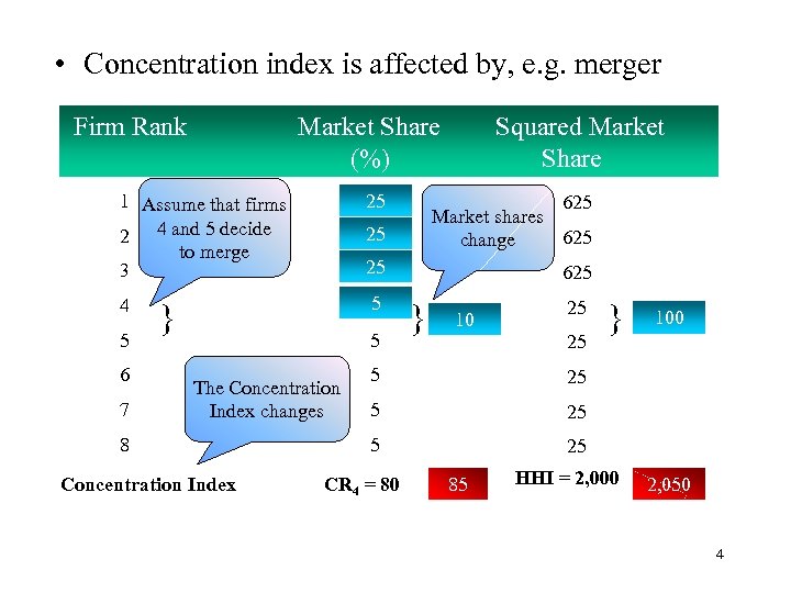• Concentration index is affected by, e. g. merger Firm Rank Market Share (%) 1 Assume that firms 2 4 and 5 decide to merge 3 25 4 5 5 6 7 25 625 Market shares 625 change 25 } 625 5 Concentration Index } 10 25 25 5 5 } 100 25 25 5 The Concentration Index changes 8 Squared Market Share 25 CR 4 = 80 85 HHI = 2, 000 2, 050 4

2. 1. 2 What is a market? • No clear consensus: To use CR 4 or HHI as an overall measure of a market’s structure, we need to be able to identify a well-defined market first. Example 1, the market for automobiles • should we include light trucks; pick-ups SUVs? Example 2, the market for soft drinks • what are the competitors for Coca Cola and Pepsi? – With whom do Mc. Donalds and Burger King compete? • Presumably define a market by closeness in substitutability of the commodities involved – how close is close? 5

Market definition (cont. ) – how homogeneous do commodities have to be? • Does wood compete with plastic? Rayon with wool? • Definition is important – without consistency concept of a market is meaningless – need indication of competitiveness of a market: affected by definition – public policy: decisions on mergers can turn on market definition • Staples/Office Depot merger rejected on market definition • Coca Cola expansion turned on market definition • Standard approach has some consistency – based upon industrial data – substitutability is production not consumption (ease of data 6 collection)

Market definition (cont. ) • Government statistical sources Census Bureau: Standard Industrial Classification (SIC) North American Industry Classification System (NAICS) • The measure of concentration varies across countries • Use of production-based statistics has limitations: – can put in different industries products that are in the same market • The international dimension is important – Boeing/Mc. Donnell-Douglas merger – relevant market for automobiles, oil, hairdressing 7

Market definition (cont. ) • Geography is important – barrier to entry if the product is expensive to transport – but customers can move • what is the relevant market for a beach resort or ski-slope? • Vertical relations between firms are important – most firms make intermediate rather than final goods – firm has to make a series of make-or-buy choices – upstream and downstream production – measures of concentration may assign firms at different stages to the same industry • do vertical relations affect underlying structure? 8

Market definition (cont. ) – Firms at different stages may also be assigned to different industries • bottlers of soft drinks: low concentration • suppliers of sift drinks: high concentration • the bottling sector is probably not competitive. • In sum: market definition poses real problems – existing methods represent a reasonable compromise 9

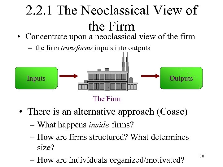2. 2. 1 The Neoclassical View of the Firm • Concentrate upon a neoclassical view of the firm – the firm transforms inputs into outputs Inputs Outputs The Firm • There is an alternative approach (Coase) – What happens inside firms? – How are firms structured? What determines size? – How are individuals organized/motivated? 10

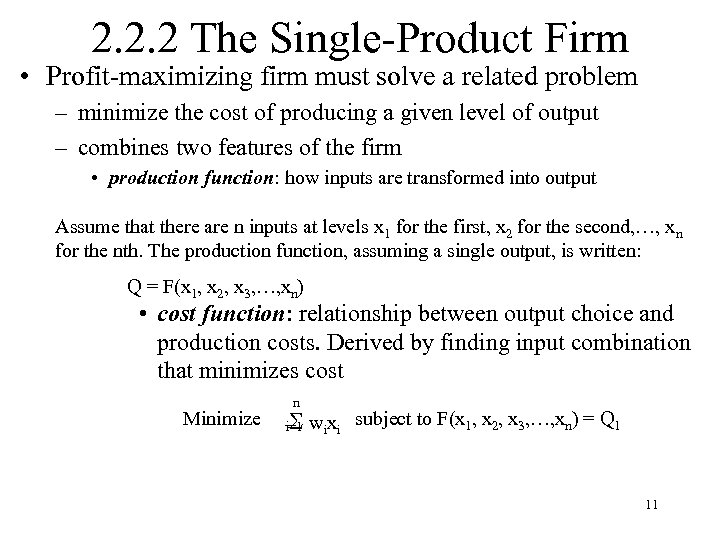2. 2. 2 The Single-Product Firm • Profit-maximizing firm must solve a related problem – minimize the cost of producing a given level of output – combines two features of the firm • production function: how inputs are transformed into output Assume that there are n inputs at levels x 1 for the first, x 2 for the second, …, xn for the nth. The production function, assuming a single output, is written: Q = F(x 1, x 2, x 3, …, xn) • cost function: relationship between output choice and production costs. Derived by finding input combination that minimizes cost Minimize n wixi subject to F(x 1, x 2, x 3, …, xn) = Q 1 i=1 11

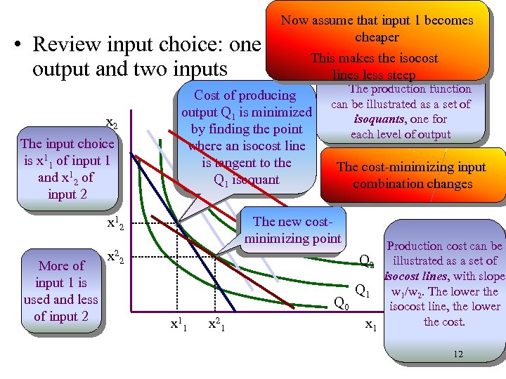Now assume that input 1 becomes cheaper This makes the isocost lines less steep The production function Cost of producing can be illustrated as a set of output Q 1 is minimized isoquants, one for by finding the point each level of output where an isocost line is tangent to the The cost-minimizing input Q 1 isoquant combination changes • Review input choice: one output and two inputs x 2 The input choice is x 11 of input 1 and x 12 of input 2 The new costminimizing point x 12 More of input 1 is used and less of input 2 x 2 2 x 11 x 21 Production cost can be Q 2 illustrated as a set of isocost lines, with slope Q 1 w 1/w 2. The lower the Q 0 isocost line, the lower the cost. x 1 12

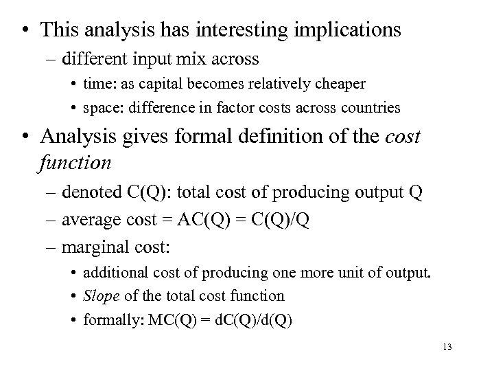• This analysis has interesting implications – different input mix across • time: as capital becomes relatively cheaper • space: difference in factor costs across countries • Analysis gives formal definition of the cost function – denoted C(Q): total cost of producing output Q – average cost = AC(Q) = C(Q)/Q – marginal cost: • additional cost of producing one more unit of output. • Slope of the total cost function • formally: MC(Q) = d. C(Q)/d(Q) 13

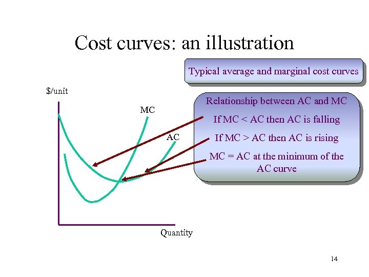Cost curves: an illustration Typical average and marginal cost curves $/unit Relationship between AC and MC MC If MC < AC then AC is falling AC If MC > AC then AC is rising MC = AC at the minimum of the AC curve Quantity 14

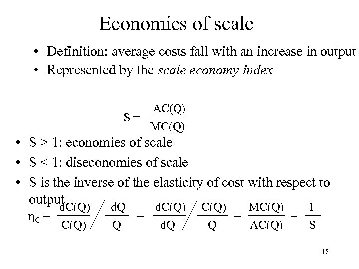Economies of scale • Definition: average costs fall with an increase in output • Represented by the scale economy index AC(Q) S= MC(Q) • S > 1: economies of scale • S < 1: diseconomies of scale • S is the inverse of the elasticity of cost with respect to output d. C(Q) d. Q d. C(Q) MC(Q) 1 h. C = C(Q) Q = d. Q Q = AC(Q) = S 15

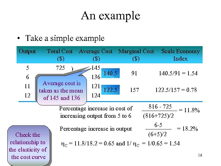An example • Take a simple example Output Total Cost Average Cost Marginal Cost Scale Economy ($) ($) Index 5 725 140. 5 91 140. 5/91 = 1. 54 6 816 136 Average cost is 11 1331 122. 5 157 122. 5/157 = 0. 78 taken as the mean 12 1488 124 of 145 and 136 816 - 725 Percentage increase in cost of = 11. 8% increasing output from 5 to 6 (816+725)/2 6 -5 Percentage increase in output = 18. 2% (6+5)/2 Check the relationship to h. C = 11. 8/18. 2 = 0. 65 and 1/ h. C = 1/0. 65 = 1. 54 the elasticity of 16 the cost curve } }

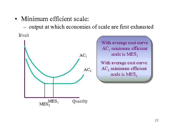• Minimum efficient scale: – output at which economies of scale are first exhausted $/unit AC 1 AC 2 MES 1 MES 2 With average cost curve AC 1 minimum efficient scale is MES 1 With average cost curve AC 2 minimum efficient scale is MES 2 Quantity 17

Natural monopoly • If the extent of the market is less than MES then the market is a natural monopoly: S > 1 in such a market. • But a natural monopoly can exist even if S < 1. Economies of scale • Sources of economies of scale – “the 60% rule”: capacity related to volume while cost is related to surface area – product specialization and the division of labor – “economies of mass reserves”: economize on inventory, maintenance, repair 18 – indivisibilities

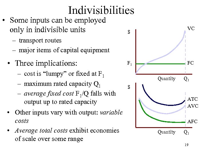Indivisibilities • Some inputs can be employed only in indivisible units VC $ – transport routes – major items of capital equipment • Three implications: – cost is “lumpy” or fixed at F 1 – maximum rated capacity Q 1 – average fixed cost F 1/Q falls with output up to rated capacity • Other inputs vary with output: variable costs • Average total costs exhibit economies of scale over some range F 1 FC Quantity Q 1 $ ATC AVC AFC Quantity Q 1 19

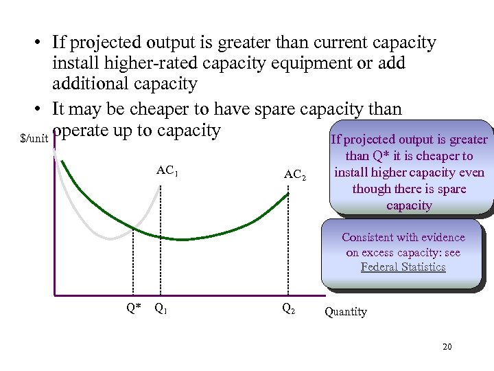• If projected output is greater than current capacity install higher-rated capacity equipment or additional capacity • It may be cheaper to have spare capacity than operate up to capacity $/unit If projected output is greater AC 1 AC 2 than Q* it is cheaper to install higher capacity even though there is spare capacity Consistent with evidence on excess capacity: see Federal Statistics Q* Q 1 Q 2 Quantity 20

Fixed costs, indivisibilities and sunk costs • Indivisibilities make scale of entry an important strategic decision: – enter large with large-scale indivisibilities: heavy overhead – enter small with smaller-scale cheaper equipment: low overhead • Some indivisible inputs can be redeployed – aircraft • Other indivisibilities are highly specialized with little value in other uses – market research expenditures – rail track between two destinations • The latter are sunk costs: nonrecoverable if production stops • Fixed costs and sunk costs affect market structure by 21 affecting entry

Multi-Product Firms • Many firms make multiple products – Ford, General Motors, 3 M etc. • What do we mean by costs and output in these cases? • How do we define average costs for these firms? – – total cost for a two-product firm is C(Q 1, Q 2) marginal cost for product 1 is MC 1 = C(Q 1, Q 2)/ Q 1 but average cost cannot be defined fully generally need a more restricted definition: ray average cost 22

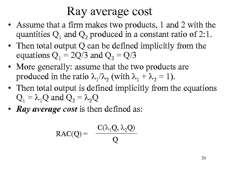Ray average cost • Assume that a firm makes two products, 1 and 2 with the quantities Q 1 and Q 2 produced in a constant ratio of 2: 1. • Then total output Q can be defined implicitly from the equations Q 1 = 2 Q/3 and Q 2 = Q/3 • More generally: assume that the two products are produced in the ratio 1/ 2 (with 1 + 2 = 1). • Then total output is defined implicitly from the equations Q 1 = 1 Q and Q 2 = 2 Q • Ray average cost is then defined as: RAC(Q) = C( 1 Q, 2 Q) Q 23

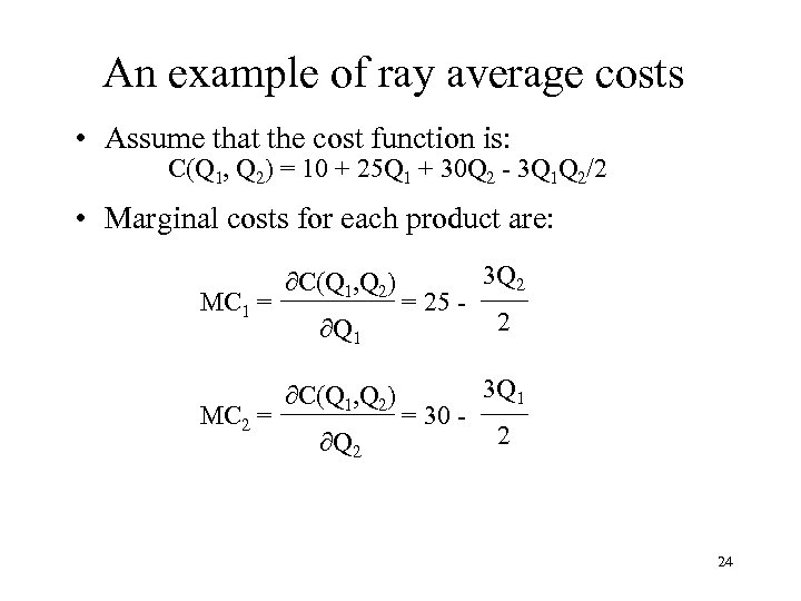An example of ray average costs • Assume that the cost function is: C(Q 1, Q 2) = 10 + 25 Q 1 + 30 Q 2 - 3 Q 1 Q 2/2 • Marginal costs for each product are: MC 1 = MC 2 = C(Q 1, Q 2) Q 1 C(Q 1, Q 2) Q 2 = 25 - = 30 - 3 Q 2 2 3 Q 1 2 24

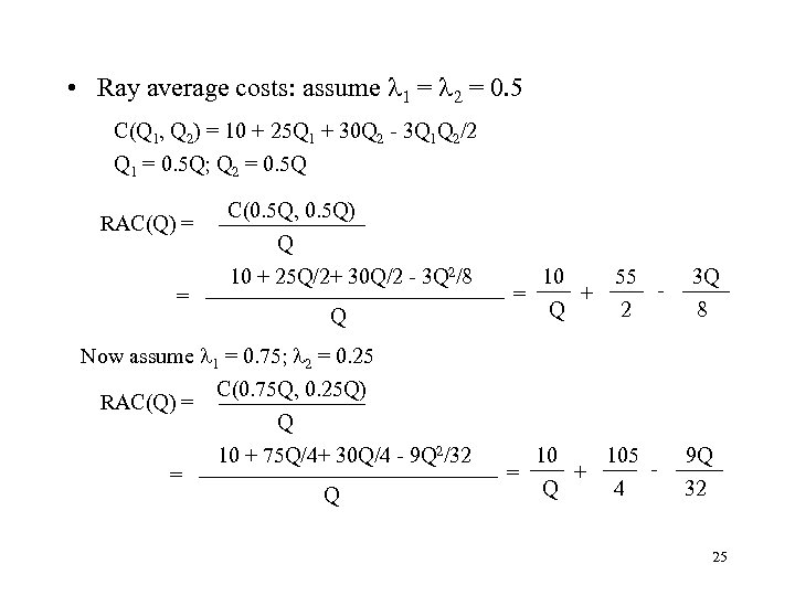• Ray average costs: assume 1 = 2 = 0. 5 C(Q 1, Q 2) = 10 + 25 Q 1 + 30 Q 2 - 3 Q 1 Q 2/2 Q 1 = 0. 5 Q; Q 2 = 0. 5 Q RAC(Q) = = C(0. 5 Q, 0. 5 Q) Q 10 + 25 Q/2+ 30 Q/2 - 3 Q 2/8 Q Now assume 1 = 0. 75; 2 = 0. 25 C(0. 75 Q, 0. 25 Q) RAC(Q) = Q 10 + 75 Q/4+ 30 Q/4 - 9 Q 2/32 = Q = 10 Q + 55 2 - 10 105 + = Q 4 3 Q 8 9 Q 32 25

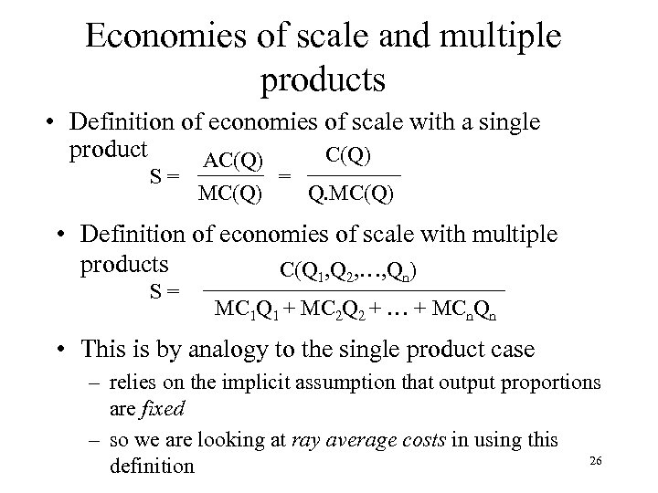Economies of scale and multiple products • Definition of economies of scale with a single product C(Q) AC(Q) S= MC(Q) = Q. MC(Q) • Definition of economies of scale with multiple products C(Q 1, Q 2, …, Qn) S= MC 1 Q 1 + MC 2 Q 2 + … + MCn. Qn • This is by analogy to the single product case – relies on the implicit assumption that output proportions are fixed – so we are looking at ray average costs in using this 26 definition

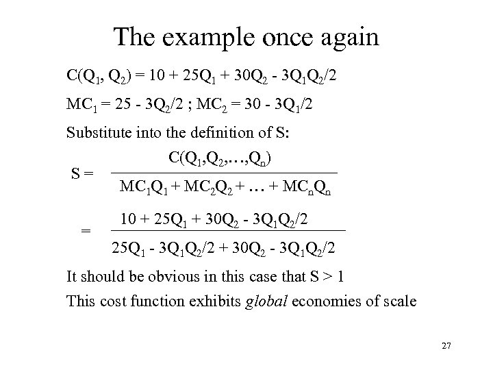The example once again C(Q 1, Q 2) = 10 + 25 Q 1 + 30 Q 2 - 3 Q 1 Q 2/2 MC 1 = 25 - 3 Q 2/2 ; MC 2 = 30 - 3 Q 1/2 Substitute into the definition of S: C(Q 1, Q 2, …, Qn) S= MC 1 Q 1 + MC 2 Q 2 + … + MCn. Qn = 10 + 25 Q 1 + 30 Q 2 - 3 Q 1 Q 2/2 25 Q 1 - 3 Q 1 Q 2/2 + 30 Q 2 - 3 Q 1 Q 2/2 It should be obvious in this case that S > 1 This cost function exhibits global economies of scale 27

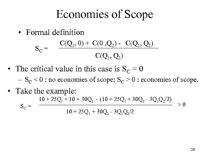Economies of Scope • Formal definition SC = C(Q 1, 0) + C(0 , Q 2) - C(Q 1, Q 2) • The critical value in this case is SC = 0 – SC < 0 : no economies of scope; SC > 0 : economies of scope. • Take the example: SC = 10 + 25 Q 1 + 10 + 30 Q 2 - (10 + 25 Q 1 + 30 Q 2 - 3 Q 1 Q 2/2) >0 10 + 25 Q 1 + 30 Q 2 - 3 Q 1 Q 2/2 28

Economies of Scope (cont. ) • Sources of economies of scope • shared inputs – same equipment for various products – shared advertising creating a brand name – marketing and R&D expenditures that are generic • cost complementarities – – – producing one good reduces the cost of producing another oil and natural gas oil and benzene computer software and computer support retailing and product promotion 29

Flexible Manufacturing • Extreme version of economies of scope • Changing the face of manufacturing • “Production units capable of producing a range of discrete products with a minimum of manual intervention” – – Benetton Custom Shoe Levi’s Mitsubishi • Production units can be switched easily with little if any cost penalty – requires close contact between design and manufacturing 30

Flexible Manufacturing (cont. ) • Take a simple model based on a spatial analogue. – There is some characteristic that distinguishes different varieties of a product • sweetness or sugar content • color • texture – This can be measured and represented as a line – Individual products can be located on this line in terms of the quantity of the characteristic that they possess – One product is chosen by the firm as its base product – All other products are variants on the base product 31

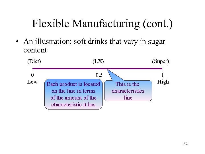Flexible Manufacturing (cont. ) • An illustration: soft drinks that vary in sugar content (Diet) (LX) (Super) 0 Low 0. 5 1 High Each product is located on the line in terms of the amount of the characteristic it has This is the characteristics line 32

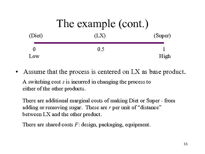The example (cont. ) (Diet) (LX) (Super) 0 Low 0. 5 1 High • Assume that the process is centered on LX as base product. A switching cost s is incurred in changing the process to either of the other products. There additional marginal costs of making Diet or Super - from adding or removing sugar. These are r per unit of “distance” between LX and the other product. There are shared costs F: design, packaging, equipment. 33

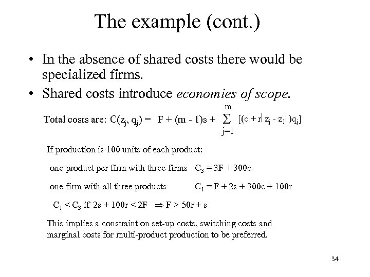The example (cont. ) • In the absence of shared costs there would be specialized firms. • Shared costs introduce economies of scope. m Total costs are: C(zj, qj) = F + (m - 1)s + [(c + r zj - z 1 )qj] j=1 If production is 100 units of each product: one product per firm with three firms C 3 = 3 F + 300 c one firm with all three products C 1 = F + 2 s + 300 c + 100 r C 1 < C 3 if 2 s + 100 r < 2 F F > 50 r + s This implies a constraint on set-up costs, switching costs and marginal costs for multi-production to be preferred. 34

Economies of scale and scope • Economies of scale and scope affect market structure but cannot be looked at in isolation. • They must be considered relative to market size. • Should see concentration decline as market size increases • For example, entry to the medical profession is going to be more extensive in Chicago than in Oxford, Miss 35

Network Externalities • Market structure is also affected by the presence of network externalities – willingness to pay by a consumer increases as the number of current consumers increase • telephones, fax, Internet, Windows software • utility from consumption increases when there are more current consumers • These markets are likely to contain a small number of firms – even if there are limited economies of scale and scope 36

The Role of Policy • Government can directly affect market structure – by limiting entry • taxi medallions in Boston and New York • airline regulation – through the patent system – by protecting competition e. g. through the Robinson -Patman Act 37

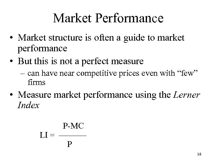Market Performance • Market structure is often a guide to market performance • But this is not a perfect measure – can have near competitive prices even with “few” firms • Measure market performance using the Lerner Index LI = P-MC P 38

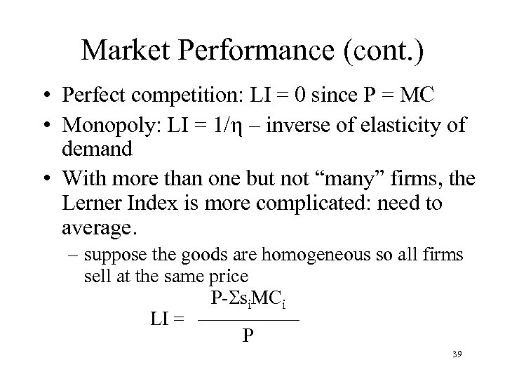Market Performance (cont. ) • Perfect competition: LI = 0 since P = MC • Monopoly: LI = 1/h – inverse of elasticity of demand • With more than one but not “many” firms, the Lerner Index is more complicated: need to average. – suppose the goods are homogeneous so all firms sell at the same price P- si. MCi LI = P 39

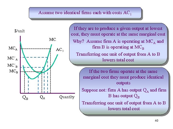Assume two identical firms each with costs AC 1 If they are to produce a given output at lowest cost, they must operate at the same marginal cost $/unit MC MCA AC 1 MC´A Why? Assume firm A is operating at MCA and firm B is operating at MCB Transferring one unit of output from A to B lowers total cost MC´B MCB If the two firms operate at the same marginal cost they must produce identical outputs QB QA Quantity Suppose not: firm A has output QA and firm B has output QB Transferring one unit of output from A to B lowers total cost 40

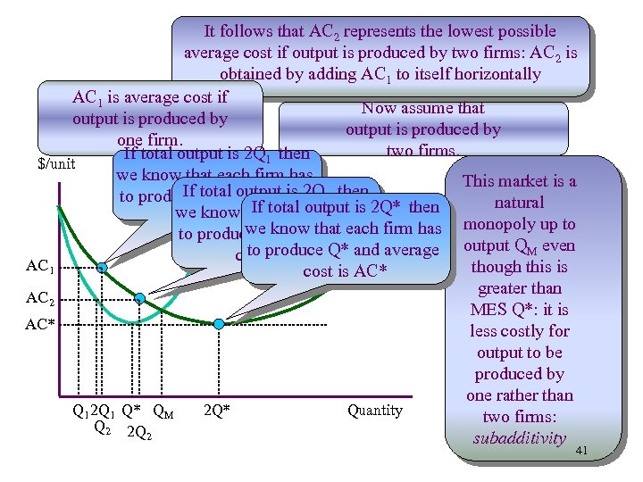It follows that AC 2 represents the lowest possible average cost if output is produced by two firms: AC 2 is obtained by adding AC 1 to itself horizontally AC 1 is average cost if Now assume that output is produced by one firm. two firms. If total output is 2 Q 1 then $/unit we know that each firm has This market is a If total output is 2 Q 2 then to produce Q 1 and average natural If each firm is we know thattotal outputhas 2 Q* then cost is AC 1 monopoly up to to. AC 1 we know average 2 firm has produce Q 2 and that each AC to produce Q* and average output QM even cost is AC 2 AC 1 though this is cost is AC* greater than AC 2 MES Q*: it is AC* less costly for output to be produced by one rather than Q 1 2 Q 1 Q* QM 2 Q* Quantity two firms: Q 2 2 Q 2 subadditivity 41

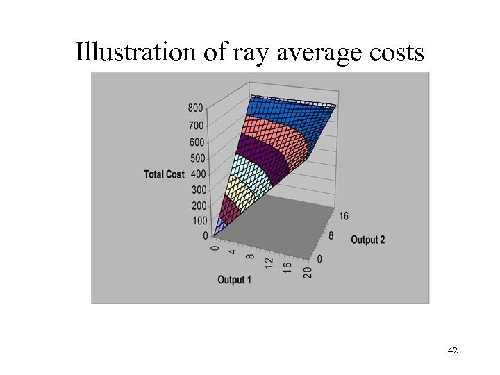Illustration of ray average costs 42