Chapter 2 Review of S and D

Chapter 2 Review of S and D • Supply Curve: • Shows quantity supplied at each possible price, ceteris paribus (c. p. ). – – – Slopes upward (positive relationship) Qs = Qs(P) Shift S Curve if change c. p. factor Movement along vs shift C. P. factors: change in cost of production; change S from bad weather. – Interpret shift S curve: change willingness to supply at each price.

Demand Curve • Shows quantity demanded at each possible price, ceteris paribus (c. p. ) – Slopes downward (negative relationship) – Qd = Qd(P) – Movement along versus shift. – C. P. factors: change income; change demand for related good. – Interpret shift D curve: change willingness to buy at each price.

Substitutes and Complements • Given two goods X and Y, if they are consumed together they are called complements and if one is used instead of the other, they are called substitutes. • Substitutes: Px Dy – When price of X , the demand for X falls. So demand for Y . – Example: beef and chicken • Complements: Px Dy – When price of X , its demand . So demand for Y also. – Example: bread and butter

Market Mechanism • Put Supply and Demand Together • Equilibrium – Point at which Qs=Qd; – Market-clearing P; • Describe re-equilibrating process by changing C. P. factor: – Increase in income causes increase in demand (shift D rightward) – At old P, Qd greater than Qs: so individuals bid up price till reach new equilibrium.

Example of Shifts in S and D • Effects of 9/11: Example 2. 4 in text. • Much destruction of office space; suggests shortage (lower vacancy rate) should drive up rental rates. • Result was different because as supply fell, demand fell also. • See Figure 2. 10

In-Class Exercise • Note in text on pg. 28: – Fact: top 20% of income distribution had 40% increase in real take-home earnings; bottom 10% of distribution had decline of 10%. • Consider: two separate labor markets for skilled and unskilled workers. Start in equilibrium for both; then show: – Unskilled workers: big S, small D – Skilled workers: small S, big D. – Outcome will explain observed trend: big increase in inequality in 1980 s and 1990 s; or, increase in working poor.

Homework Assignment • Consider the two separate markets for peanut butter and jelly. Assume that the two products are complements for consumers. – 1. Sketch and describe the initial equilibrium in both markets. – 2. Show the effect of new health warnings about all the fat in peanut butter in first the market for peanut butter and then in the market for jelly. – 3. Draw and label completely and describe in words.

Elasticity • Definition: % Qd in response to a 1% P • Or: % Qd / % P • What is % ? Absolute change in variable divided by original level of variable. • Ep = ( Qd/Q) / ( P/P) • = (P/Q) ( Q/ P) • Remember: ( Q/ P) is 1/slope. • Ep = price elasticity of demand; usually negative.

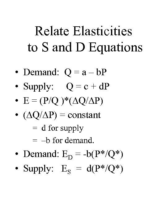Relate Elasticities to S and D Equations • • Demand: Q = a – b. P Supply: Q = c + d. P E = (P/Q )*( Q/ P) = constant = d for supply = –b for demand. • Demand: ED = -b(P*/Q*) • Supply: ES = d(P*/Q*)

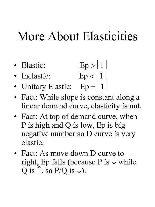More About Elasticities Elastic: Ep 1 Inelastic: Ep 1 Unitary Elastic: Ep 1 Fact: While slope is constant along a linear demand curve, elasticity is not. • Fact: At top of demand curve, when P is high and Q is low, Ep is big negative number so D curve is very elastic. • Fact: As move down D curve to right, Ep falls (because P is while Q is , so P/Q is ). • •

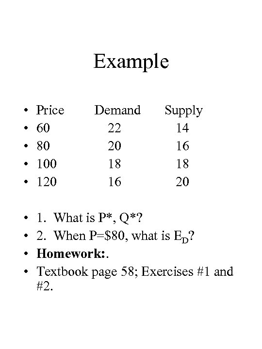Example • • • Price 60 80 100 120 • • 1. What is P*, Q*? 2. When P=$80, what is ED? Homework: . Textbook page 58; Exercises #1 and #2. Demand 22 20 18 16 Supply 14 16 18 20

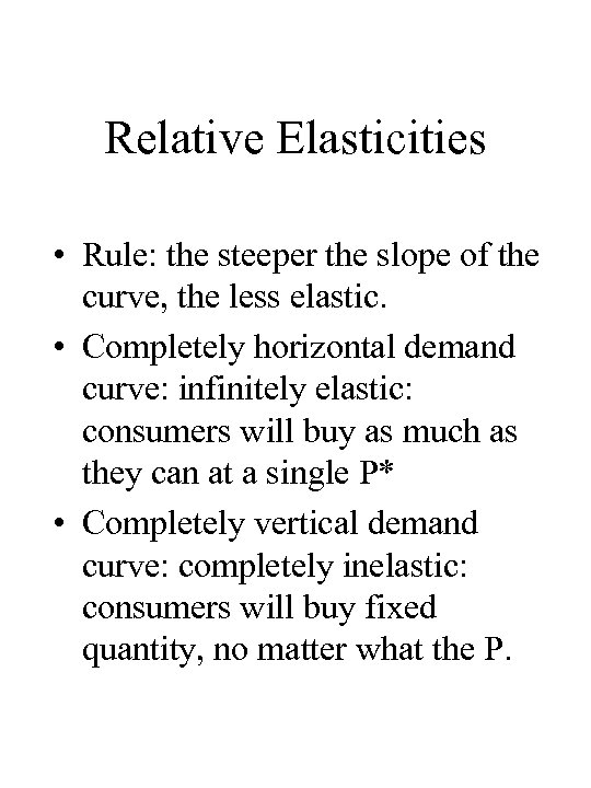Relative Elasticities • Rule: the steeper the slope of the curve, the less elastic. • Completely horizontal demand curve: infinitely elastic: consumers will buy as much as they can at a single P* • Completely vertical demand curve: completely inelastic: consumers will buy fixed quantity, no matter what the P.

Nearly Horizontal Demand Curve • Elasticity approaches infinity: Recall: 1/slope = Q/ P • If nearly flat curve: small P causes a huge Q. This is same as: huge / small , which equals a very big number. • This will help you remember elasticity for completely flat versus completely vertical.

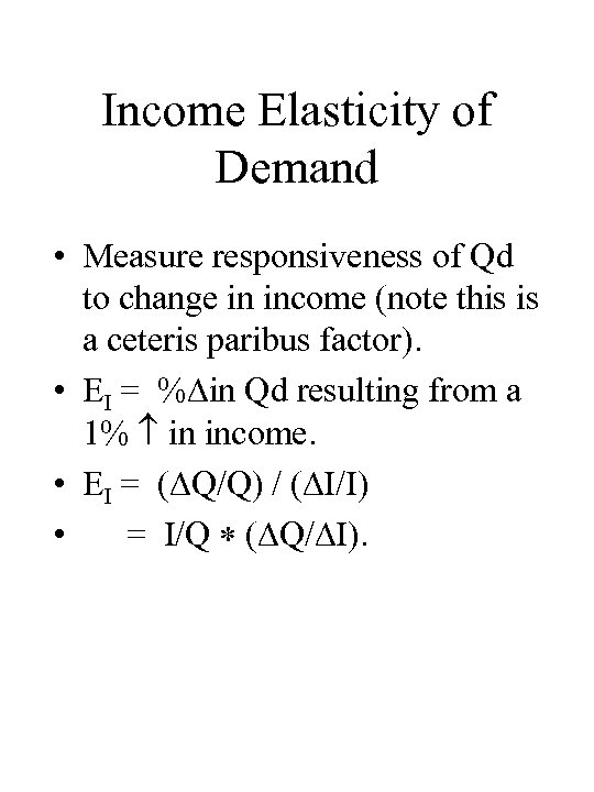Income Elasticity of Demand • Measure responsiveness of Qd to change in income (note this is a ceteris paribus factor). • EI = % in Qd resulting from a 1% in income. • EI = ( Q/Q) / ( I/I) • = I/Q ( Q/ I).

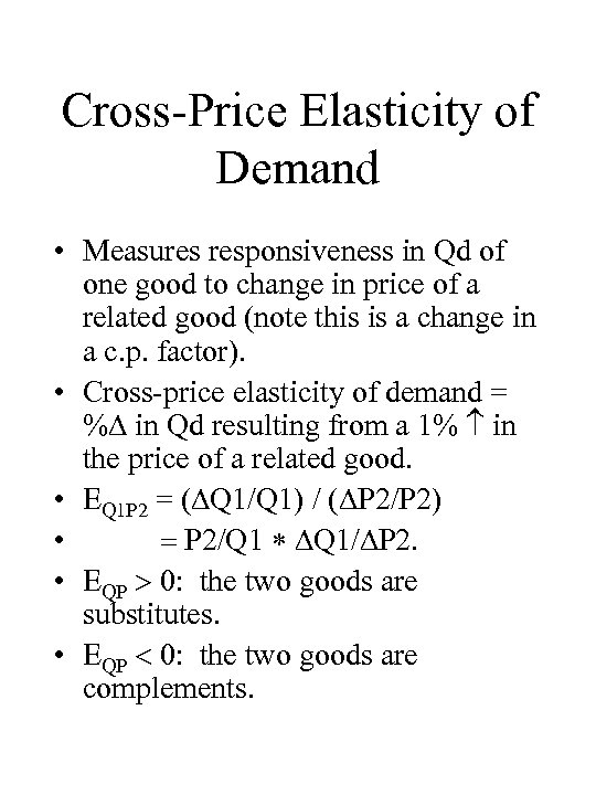Cross-Price Elasticity of Demand • Measures responsiveness in Qd of one good to change in price of a related good (note this is a change in a c. p. factor). • Cross-price elasticity of demand = % in Qd resulting from a 1% in the price of a related good. • EQ 1 P 2 = ( Q 1/Q 1) / ( P 2/P 2) • P 2/Q 1 Q 1/ P 2. • EQP 0: the two goods are substitutes. • EQP 0: the two goods are complements.

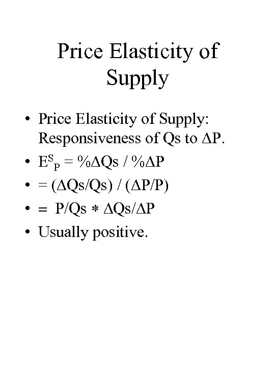Price Elasticity of Supply • Price Elasticity of Supply: Responsiveness of Qs to P. • ESP = % Qs / % P • = ( Qs/Qs) / ( P/P) • P/Qs Qs/ P • Usually positive.

Wage Elasticity of Supply • Measures responsiveness of Qs to changes in the cost of labor (a ceteris paribus factor). • ESW = % Qs / % W • = ( Qs/Qs) / ( W/W) • W/Qs Qs/ W. • Usually negative. • Remember: W cost of production.

Example • • Qs = 3 + 12 P Qd = 19 – 4 P 1. Find P* by setting Qs=Qd. 2. Find Q* by putting P* into either Qs or Qd. • Solve for Ep of demand at equilibrium: • EDP* = (P*/Q*) ( Q/ P)

Short-Run versus Long-run Elasticities • Focal point: how much time do sellers and consumers have to respond (in their Qs and Qd) to changes in price? • In general: LR adjustment is more full, free adjustment so that LR elasticity is larger; BUT not true all the time. • Key factors: – Durability. – Availability of substitutes – % of consumer’s budget

Government Price Controls • Key: If government sets P so that there is no single P for which Qs=Qd, then there will be a shortage or surplus. • Be able to show the Qs and Qd for any price. • Price ceiling: prevents price from rising above the ceiling. • Price floor: prevents price from falling below floor.

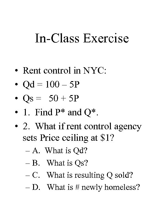In-Class Exercise • • • Rent control in NYC: Qd = 100 – 5 P Qs = 50 + 5 P 1. Find P* and Q*. 2. What if rent control agency sets Price ceiling at $1? – A. – B. – C. – D. What is Qd? What is Qs? What is resulting Q sold? What is # newly homeless?