6226436fa37867d78b6c64ce950e20cb.ppt
- Количество слайдов: 32
CHAPTER 2 - PROBABILITY CONCEPTS • Types of Probability • Fundamentals of Probability • Statistical Independence and Dependence • Bayes Theorem QP 5013 – PROBABILITY CONCEPTS 1
Introduction • Life is uncertain! • We must deal with risk! • A probability is a numerical statement about the likelihood that an event will occur QP 5013 – PROBABILITY CONCEPTS 2
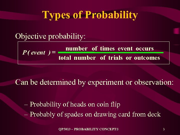
Types of Probability Objective probability: P ( event ) = number of times event occurs total number of trials or outcomes Can be determined by experiment or observation: – Probability of heads on coin flip – Probably of spades on drawing card from deck QP 5013 – PROBABILITY CONCEPTS 3
Types of Probability (cont. ) • Subjective probability is an estimate based on personal belief, experience, or knowledge of a situation: • It is often the only means available for making probabilistic estimates. • Frequently used in making business decisions. • Different people often arrive at different subjective probabilities. ü Judgment of expert ü Opinion polls ü Delphi method QP 5013 – PROBABILITY CONCEPTS 4
Fundamentals of Probability Outcomes and Events • An experiment is an activity that results in one of several possible outcomes which are termed events. • The probability of an event is always greater than or equal to zero and less than or equal to one: 0 P(event) 1 • The probabilities of all the events included in an experiment must sum to one. • The events in an experiment are mutually exclusive if only one can occur at a time. • The probabilities of mutually exclusive events sum to one. QP 5013 – PROBABILITY CONCEPTS 5
Fundamentals of Probability Distributions • A frequency distribution is an organization of numerical data about the events in an experiment. • A list of corresponding probabilities for each event is referred to as a probability distribution. • If two or more events cannot occur at the same time they are termed mutually exclusive. • A set of events is collectively exhaustive when it includes all the events that can occur in an experiment. QP 5013 – PROBABILITY CONCEPTS 6
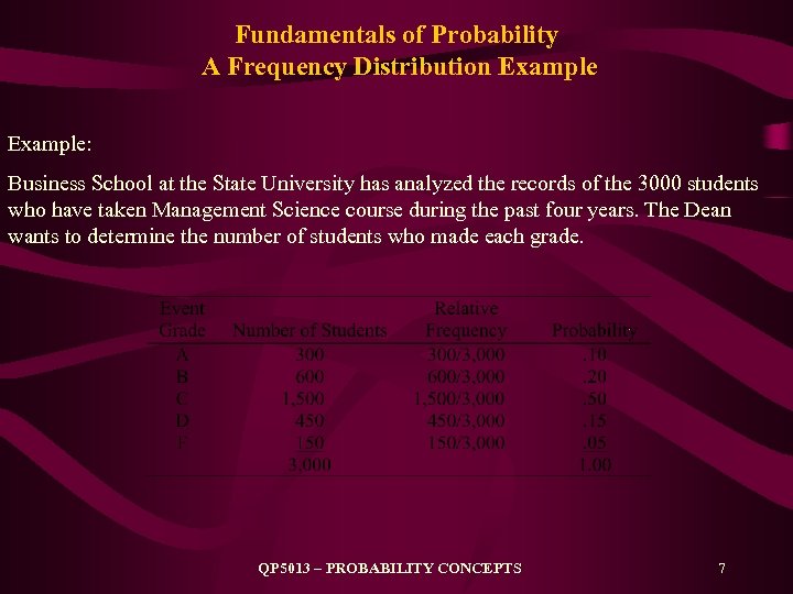
Fundamentals of Probability A Frequency Distribution Example: Business School at the State University has analyzed the records of the 3000 students who have taken Management Science course during the past four years. The Dean wants to determine the number of students who made each grade. QP 5013 – PROBABILITY CONCEPTS 7
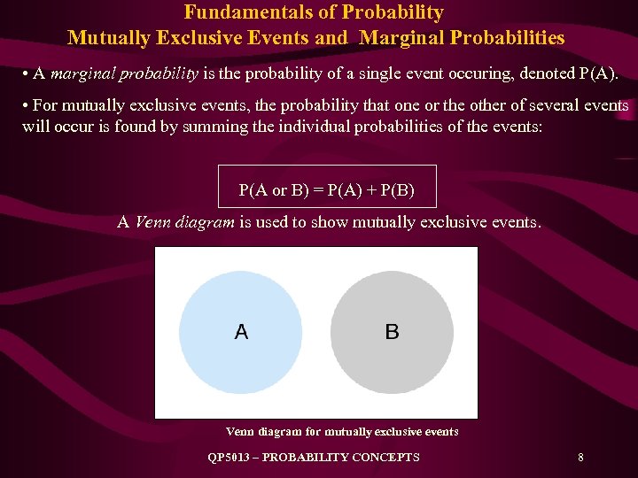
Fundamentals of Probability Mutually Exclusive Events and Marginal Probabilities • A marginal probability is the probability of a single event occuring, denoted P(A). • For mutually exclusive events, the probability that one or the other of several events will occur is found by summing the individual probabilities of the events: P(A or B) = P(A) + P(B) A Venn diagram is used to show mutually exclusive events. Venn diagram for mutually exclusive events QP 5013 – PROBABILITY CONCEPTS 8
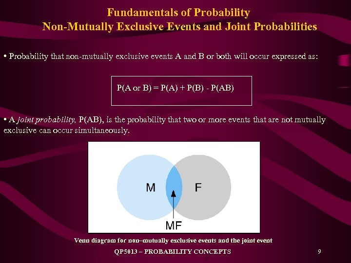
Fundamentals of Probability Non-Mutually Exclusive Events and Joint Probabilities • Probability that non-mutually exclusive events A and B or both will occur expressed as: P(A or B) = P(A) + P(B) - P(AB) • A joint probability, P(AB), is the probability that two or more events that are not mutually exclusive can occur simultaneously. Venn diagram for non–mutually exclusive events and the joint event QP 5013 – PROBABILITY CONCEPTS 9
Statistical Independence and Dependence Independent Events • A succession of events that do not affect each other are independent. • The probability of independent events occurring in a succession is computed by multiplying the probabilities of each event. • A conditional probability is the probability that an event will occur given that another event has already occurred, denoted as P(A B). If events A and B are independent, then: 1. P(AB) = P(A) P(B) 2. P(A B) = P(A) QP 5013 – PROBABILITY CONCEPTS 10
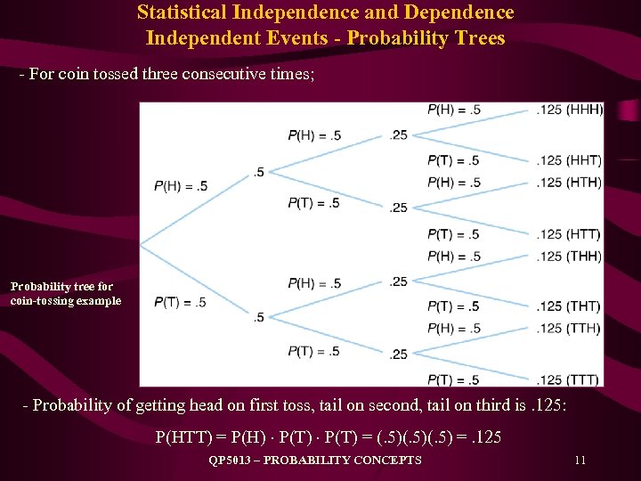
Statistical Independence and Dependence Independent Events - Probability Trees - For coin tossed three consecutive times; Probability tree for coin-tossing example - Probability of getting head on first toss, tail on second, tail on third is. 125: P(HTT) = P(H) P(T) = (. 5)(. 5) =. 125 QP 5013 – PROBABILITY CONCEPTS 11
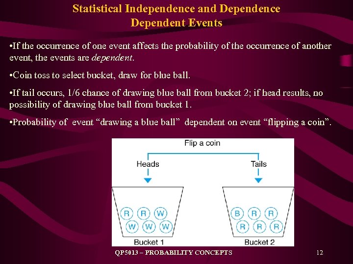
Statistical Independence and Dependence Dependent Events • If the occurrence of one event affects the probability of the occurrence of another event, the events are dependent. • Coin toss to select bucket, draw for blue ball. • If tail occurs, 1/6 chance of drawing blue ball from bucket 2; if head results, no possibility of drawing blue ball from bucket 1. • Probability of event “drawing a blue ball” dependent on event “flipping a coin”. QP 5013 – PROBABILITY CONCEPTS 12
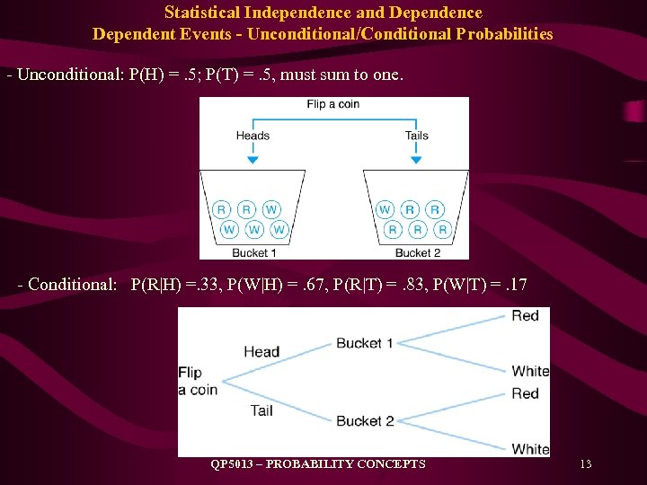
Statistical Independence and Dependence Dependent Events - Unconditional/Conditional Probabilities - Unconditional: P(H) =. 5; P(T) =. 5, must sum to one. - Conditional: P(R H) =. 33, P(W H) =. 67, P(R T) =. 83, P(W T) =. 17 QP 5013 – PROBABILITY CONCEPTS 13
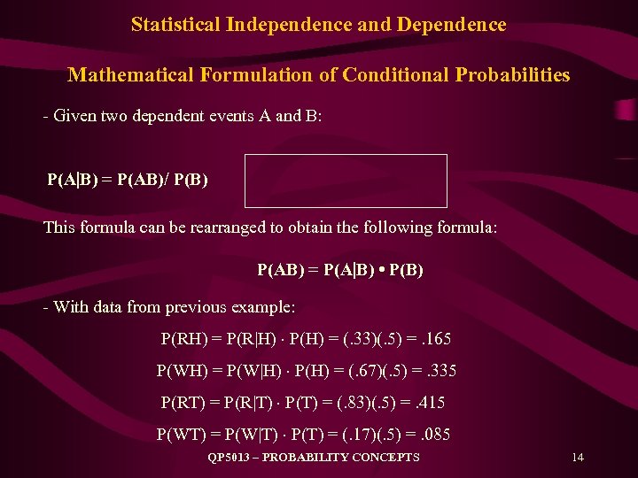
Statistical Independence and Dependence Mathematical Formulation of Conditional Probabilities - Given two dependent events A and B: P(A B) = P(AB)/ P(B) This formula can be rearranged to obtain the following formula: P(AB) = P(A B) • P(B) - With data from previous example: P(RH) = P(R H) P(H) = (. 33)(. 5) =. 165 P(WH) = P(W H) P(H) = (. 67)(. 5) =. 335 P(RT) = P(R T) P(T) = (. 83)(. 5) =. 415 P(WT) = P(W T) P(T) = (. 17)(. 5) =. 085 QP 5013 – PROBABILITY CONCEPTS 14
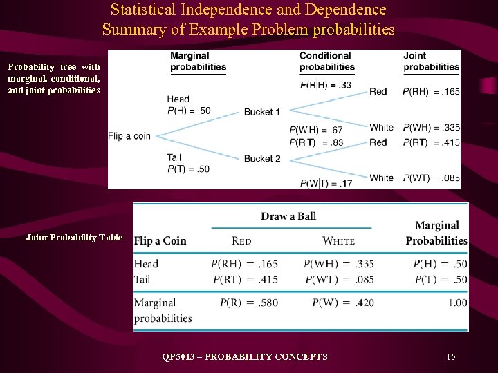
Statistical Independence and Dependence Summary of Example Problem probabilities Probability tree with marginal, conditional, and joint probabilities Joint Probability Table QP 5013 – PROBABILITY CONCEPTS 15
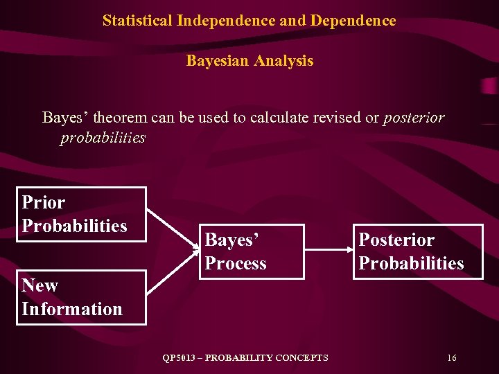
Statistical Independence and Dependence Bayesian Analysis Bayes’ theorem can be used to calculate revised or posterior probabilities Prior Probabilities Bayes’ Process Posterior Probabilities New Information QP 5013 – PROBABILITY CONCEPTS 16
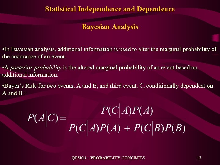
Statistical Independence and Dependence Bayesian Analysis • In Bayesian analysis, additional information is used to alter the marginal probability of the occurance of an event. • A posterior probability is the altered marginal probability of an event based on additional information. • Bayes’s Rule for two events, A and B, and third event, C, conditionally dependent on A and B : QP 5013 – PROBABILITY CONCEPTS 17
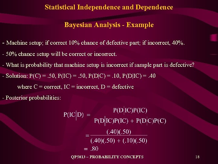
Statistical Independence and Dependence Bayesian Analysis - Example - Machine setup; if correct 10% chance of defective part; if incorrect, 40%. - 50% chance setup will be correct or incorrect. - What is probability that machine setup is incorrect if sample part is defective? - Solution: P(C) =. 50, P(IC) =. 50, P(D|C) =. 10, P(D|IC) =. 40 where C = correct, IC = incorrect, D = defective - Posterior probabilities: QP 5013 – PROBABILITY CONCEPTS 18
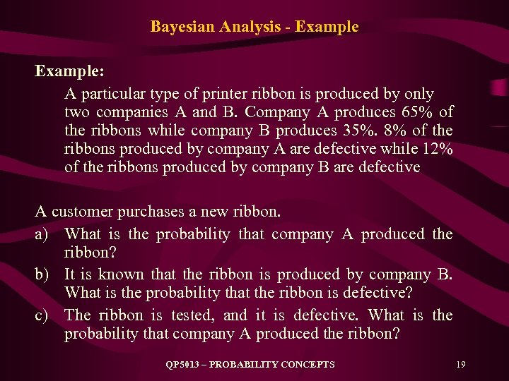
Bayesian Analysis - Example: A particular type of printer ribbon is produced by only two companies A and B. Company A produces 65% of the ribbons while company B produces 35%. 8% of the ribbons produced by company A are defective while 12% of the ribbons produced by company B are defective A customer purchases a new ribbon. a) What is the probability that company A produced the ribbon? b) It is known that the ribbon is produced by company B. What is the probability that the ribbon is defective? c) The ribbon is tested, and it is defective. What is the probability that company A produced the ribbon? QP 5013 – PROBABILITY CONCEPTS 19
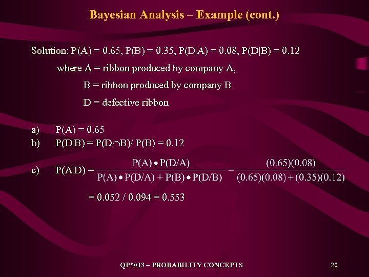
Bayesian Analysis – Example (cont. ) Solution: P(A) = 0. 65, P(B) = 0. 35, P(D|A) = 0. 08, P(D|B) = 0. 12 where A = ribbon produced by company A, B = ribbon produced by company B D = defective ribbon a) b) P(A) = 0. 65 P(D|B) = P(D B)/ P(B) = 0. 12 c) P(A|D) = = 0. 052 / 0. 094 = 0. 553 QP 5013 – PROBABILITY CONCEPTS 20
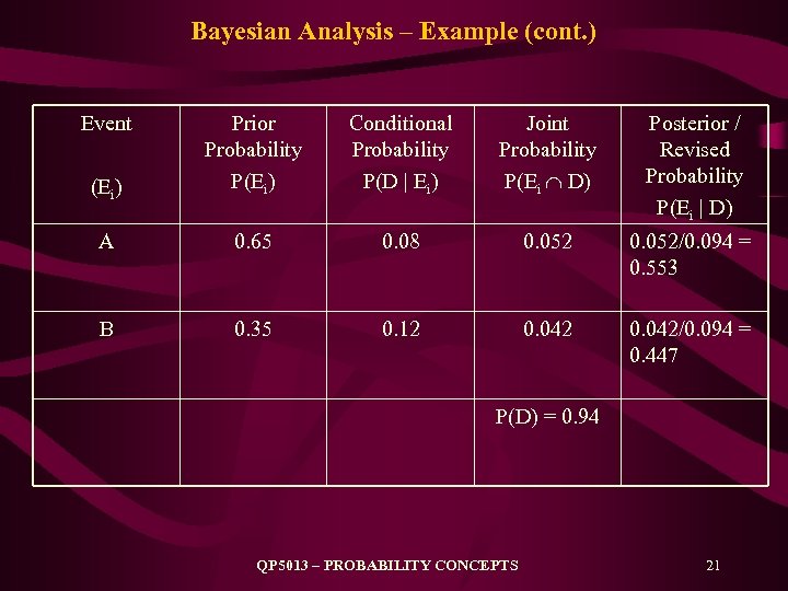
Bayesian Analysis – Example (cont. ) Event (Ei) Prior Probability P(Ei) Conditional Probability P(D | Ei) Joint Probability P(Ei D) Posterior / Revised Probability P(Ei | D) A 0. 65 0. 08 0. 052/0. 094 = 0. 553 B 0. 35 0. 12 0. 042/0. 094 = 0. 447 P(D) = 0. 94 QP 5013 – PROBABILITY CONCEPTS 21
Expected Value Random Variables - When the values of variables occur in no particular order or sequence, the variables are referred to as random variables. - Random variables are represented symbolically by a letter x, y, z, etc. - Although exact values of random variables are not known prior to events, it is possible to assign a probability to the occurrence of possible values. QP 5013 – PROBABILITY CONCEPTS 22
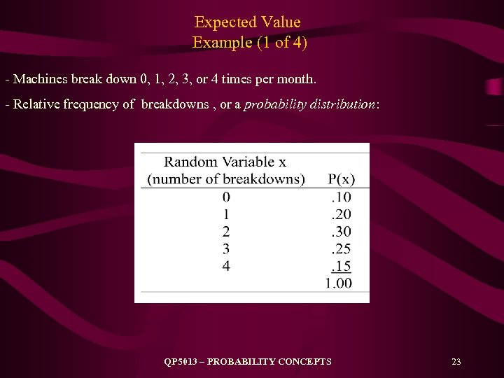
Expected Value Example (1 of 4) - Machines break down 0, 1, 2, 3, or 4 times per month. - Relative frequency of breakdowns , or a probability distribution: QP 5013 – PROBABILITY CONCEPTS 23
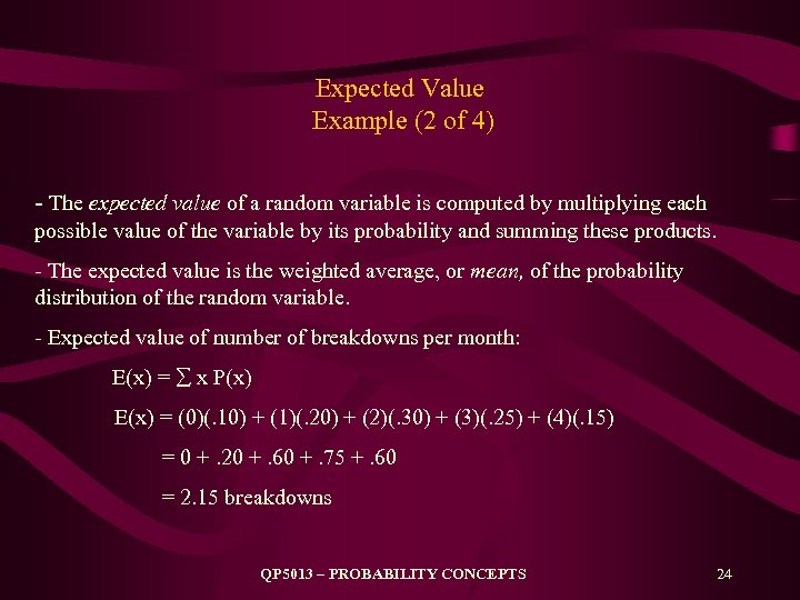
Expected Value Example (2 of 4) - The expected value of a random variable is computed by multiplying each possible value of the variable by its probability and summing these products. - The expected value is the weighted average, or mean, of the probability distribution of the random variable. - Expected value of number of breakdowns per month: E(x) = x P(x) E(x) = (0)(. 10) + (1)(. 20) + (2)(. 30) + (3)(. 25) + (4)(. 15) = 0 +. 20 +. 60 +. 75 +. 60 = 2. 15 breakdowns QP 5013 – PROBABILITY CONCEPTS 24
Expected Value Example (3 of 4) - Variance is a measure of the dispersion of random variable values about the mean. - Variance computed as follows: 1. Square each value, x 2. Multiply square of each value by the probability of each value and sum it. 3. Subtract square of mean from the value obtained in step 2 - General formula: Variance, 2 = [xi - E(xi)] 2 P(xi) = x 2 P(x) – [E(x)]2 QP 5013 – PROBABILITY CONCEPTS 25
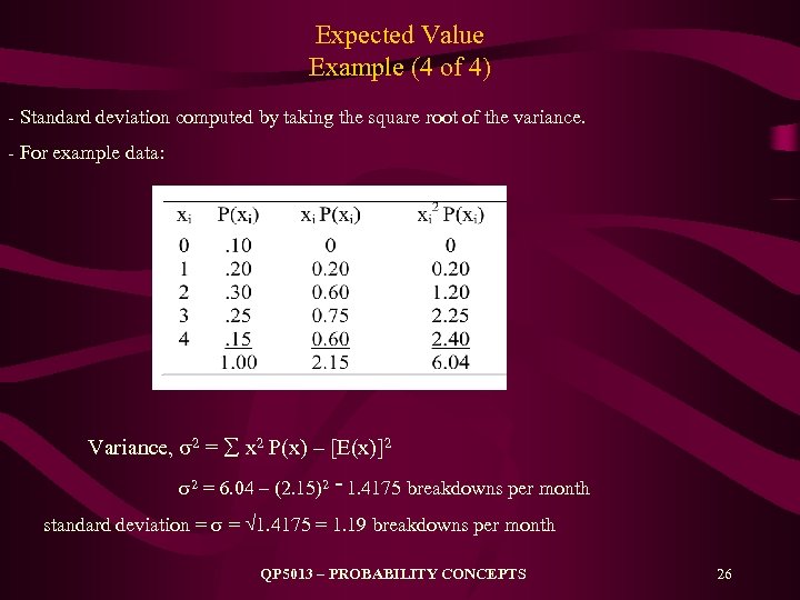
Expected Value Example (4 of 4) - Standard deviation computed by taking the square root of the variance. - For example data: Variance, 2 = x 2 P(x) – [E(x)]2 2 = 6. 04 – (2. 15)2 = 1. 4175 breakdowns per month standard deviation = = 1. 4175 = 1. 19 breakdowns per month QP 5013 – PROBABILITY CONCEPTS 26
The Normal Distribution Continuous Random Variables • A continuous random variable can take on an infinite number of values within some interval. • Continuous random variables have values that are not specifically countable and are often fractional. • Cannot assign a unique probability to each value of a continuous random variable. • In a continuous probability distribution the probability refers to a value of the random variable being within some range. QP 5013 – PROBABILITY CONCEPTS 27
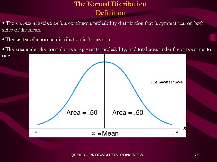
The Normal Distribution Definition • The normal distribution is a continuous probability distribution that is symmetrical on both sides of the mean. • The center of a normal distribution is its mean . • The area under the normal curve represents probability, and total area under the curve sums to one. The normal curve QP 5013 – PROBABILITY CONCEPTS 28
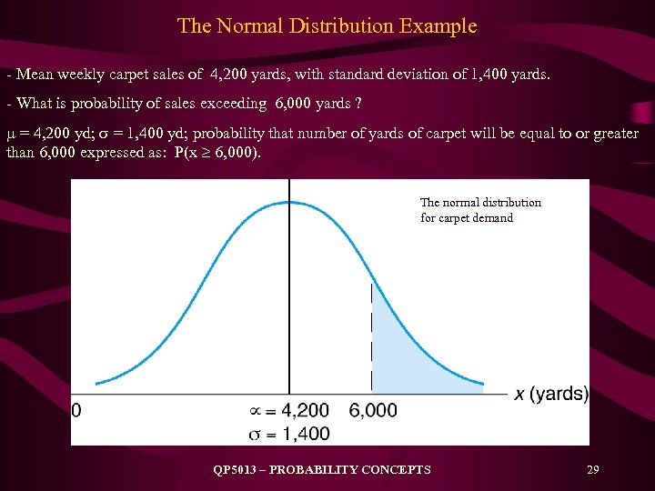
The Normal Distribution Example - Mean weekly carpet sales of 4, 200 yards, with standard deviation of 1, 400 yards. - What is probability of sales exceeding 6, 000 yards ? = 4, 200 yd; = 1, 400 yd; probability that number of yards of carpet will be equal to or greater than 6, 000 expressed as: P(x 6, 000). The normal distribution for carpet demand QP 5013 – PROBABILITY CONCEPTS 29
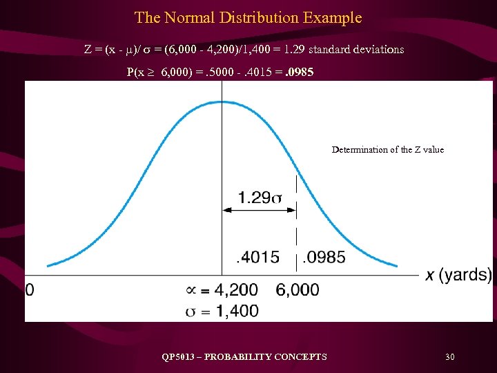
The Normal Distribution Example Z = (x - )/ = (6, 000 - 4, 200)/1, 400 = 1. 29 standard deviations P(x 6, 000) =. 5000 -. 4015 =. 0985 Determination of the Z value QP 5013 – PROBABILITY CONCEPTS 30
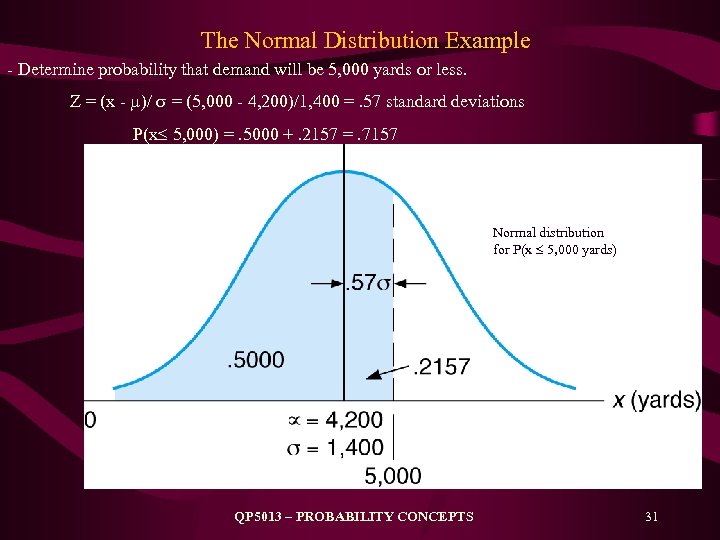
The Normal Distribution Example - Determine probability that demand will be 5, 000 yards or less. Z = (x - )/ = (5, 000 - 4, 200)/1, 400 =. 57 standard deviations P(x 5, 000) =. 5000 +. 2157 =. 7157 Normal distribution for P(x 5, 000 yards) QP 5013 – PROBABILITY CONCEPTS 31
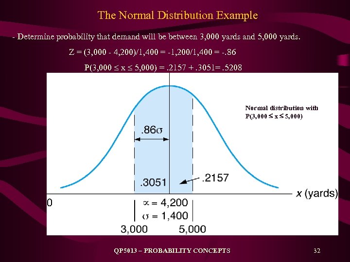
The Normal Distribution Example - Determine probability that demand will be between 3, 000 yards and 5, 000 yards. Z = (3, 000 - 4, 200)/1, 400 = -1, 200/1, 400 = -. 86 P(3, 000 x 5, 000) =. 2157 +. 3051=. 5208 Normal distribution with P(3, 000 x 5, 000) QP 5013 – PROBABILITY CONCEPTS 32
6226436fa37867d78b6c64ce950e20cb.ppt