

ff3d608bc4cf7100ba9b073ec96ef274.ppt
- Количество слайдов: 125
 Chapter 2 -OPTIMIZATION G. Anuradha
 Contents • Derivative-based Optimization – – Descent Methods The Method of Steepest Descent Classical Newton’s Method Step Size Determination • Derivative-free Optimization – – Genetic Algorithms Simulated Annealing Random Search Downhill Simplex Search
 What is Optimization? • Choosing the best element from some set of available alternatives • Solving problems in which one seeks to minimize or maximize a real function
 ----------------1 subject to gj(x 1,") Notation of Optimization Optimize y=f(x 1, x 2…. xn) ----------------1 subject to gj(x 1, x 2…xn) ≤ / ≥ /= bj -----------2 where j=1, 2, …. n Eqn: 1 is objective function Eqn: 2 a set of constraints imposed on the solution. x 1, x 2…xn are the set of decision variables Note: - The problem is either to maximize or minimize the value of objective function.
Notation of Optimization Optimize y=f(x 1, x 2…. xn) ----------------1 subject to gj(x 1, x 2…xn) ≤ / ≥ /= bj -----------2 where j=1, 2, …. n Eqn: 1 is objective function Eqn: 2 a set of constraints imposed on the solution. x 1, x 2…xn are the set of decision variables Note: - The problem is either to maximize or minimize the value of objective function.


 Complicating factors in optimization 1. Existence of multiple decision variables 2. Complex nature of the relationships between the decision variables and the associated income 3. Existence of one or more complex constraints on the decision variables
 Types of optimization • Constraint: - Solution is arrived at by maximizing or minimizing the objective function • Unconstraint: - No constraints are imposed on the decision variables and differential calculus can be used to analyze them
 Least Square Methods for System Identification • System Identification: - Determining a mathematical model for an unknown system by observing the input-output data pairs • System identification is required – To predict a system behavior – To explain the interactions and relationship between inputs and outputs – To design a controller • System identification – Structure identification – Parameter identification
 Structure identification • Apply a priori knowledge about the target system to determine a class of models within which the search for the most suitable model is conducted • y=f(u; θ) y – model’s output u – Input Vector θ – parameter vector
 Parameter Identification • Structure of the model is known and optimization techniques are applied to determine the parameter vector θ= θ
 Block diagram of parameter identification
 Parameter identification • An input ui is applied to both the system and the model • Difference between the target system’s output yi and model’s output yi is used to update a parameter vector θ to minimize the difference • System identification is not a one-pass process; it needs to do both structure and parameter identification repeatedly
 Classification of Optimization algorithms • Derivative-based algorithms: • Derivative-free algorithms
 Characteristics of derivative free algorithm 1. Derivative freeness: - repeated evaluation of objective function 2. Intuitive guidelines: - concepts are based on nature’s wisdom, such as evolution and thermodynamics 3. Slower 4. Flexibility 5. Randomness: - global optimizers 6. Analytic Opacity: -knowledge about them are based on empirical studies 7. Iterative nature: -
 Characteristics of derivative free algorithm • Stopping condition of iteration: - let k denote an iteration count and fk denote the best objective function obtained at count k. stopping condition depends on – Computation time – Optimization goal; – Minimal Improvement – Minimal relative improvement
 Basics of Matrix Manipulation and Calculus •
 Basics of Matrix Manipulation and Calculus •
 Gradient of a Scalar Function •
 Jacobian of a Vector Function •
 Least Square Estimator • Method of least squares is a standard approach to approximate solution of overdetermined systems. • Least Squares- Overall solution minimizes the sum of the squares of the errors made in solving every single equation • Application—Data Fitting
 Types of Least Squares • Least Squares – Linear: - It is a linear combination of parameters. – The model may represent a straight line, a parabola or any other linear combination of functions – Non-Linear: - the parameters appear as functions, such as β 2, eβx. If the derivatives are either constant or depend only on the values of the independent variable, the model is linear else non-linear.
 Differences between Linear and Non-Linear Least Squares Linear Non-Linear Algorithms Does not require initial values Algorithms Require Initial values Globally concave; Non convergence is a common issue not an issue Normally solved using direct methods Usually an iterative process Solution is unique Multiple minima in the sum of squares Yields unbiased estimates even when errors are uncorrelated with predictor values Yields biased estimates
 Linear regression with one variable Model representatio n Machine Learning
 500 400 300 Price 200 (in 1000 s of dollars)") Housing Prices (Portland, OR) 500 400 300 Price 200 (in 1000 s of dollars) 100 0 0 Supervised Learning 500 1000 1500 2000 Size (feet 2) 2500 Regression Problem Given the “right answer” for Predict real-valued output each example in the data. 3000
Housing Prices (Portland, OR) 500 400 300 Price 200 (in 1000 s of dollars) 100 0 0 Supervised Learning 500 1000 1500 2000 Size (feet 2) 2500 Regression Problem Given the “right answer” for Predict real-valued output each example in the data. 3000
 Size in feet 2 (x) 2104 1416") Training set of housing prices (Portland, OR) Size in feet 2 (x) 2104 1416 1534 852 … Price ($) in 1000's (y) 460 232 315 178 … Notation: m = Number of training examples x’s = “input” variable / features y’s = “output” variable / “target” variable
Training set of housing prices (Portland, OR) Size in feet 2 (x) 2104 1416 1534 852 … Price ($) in 1000's (y) 460 232 315 178 … Notation: m = Number of training examples x’s = “input” variable / features y’s = “output” variable / “target” variable
 How do we represent h ? Training Set Learning Algorithm Size of house h Estimate d price Linear regression with one variable. Univariate linear regression.

 Linear regression with one variable Cost function Machine Learning
 2104 1416 1534 852 … Hypothesis: ‘s:") Training Set Size in feet 2 (x) 2104 1416 1534 852 … Hypothesis: ‘s: Parameters How to choose ‘s ? Price ($) in 1000's (y) 460 232 315 178 …
Training Set Size in feet 2 (x) 2104 1416 1534 852 … Hypothesis: ‘s: Parameters How to choose ‘s ? Price ($) in 1000's (y) 460 232 315 178 …
 3 3 3 2 2 2 1 1 1 0 0 1 2 3
 y x Idea: Choose so that is close to for our training examples

 Linear regression with one variable Machine Learning Cost function intuition I
 Simplified Hypothesis: Parameters: Cost Function: Goal:
 (function of the parameter )") (for fixed , this is a function of x) (function of the parameter ) 3 3 2 2 1 1 y 0 0 1 x 2 3 0 -0. 5 0 0. 5 1 1. 5 2 2. 5
(for fixed , this is a function of x) (function of the parameter ) 3 3 2 2 1 1 y 0 0 1 x 2 3 0 -0. 5 0 0. 5 1 1. 5 2 2. 5
 (function of the parameter )") (for fixed , this is a function of x) (function of the parameter ) 3 3 2 2 1 1 y 0 0 1 x 2 3 0 -0. 5 0 0. 5 1 1. 5 2 2. 5
(for fixed , this is a function of x) (function of the parameter ) 3 3 2 2 1 1 y 0 0 1 x 2 3 0 -0. 5 0 0. 5 1 1. 5 2 2. 5
 (function of the parameter )") (for fixed , this is a function of x) (function of the parameter ) 3 3 2 2 1 1 y 0 0 1 x 2 3 0 -0. 5 0 0. 5 1 1. 5 2 2. 5
(for fixed , this is a function of x) (function of the parameter ) 3 3 2 2 1 1 y 0 0 1 x 2 3 0 -0. 5 0 0. 5 1 1. 5 2 2. 5

 Linear regression with one variable Machine Learning Cost function intuition II
 Hypothesis: Parameters: Cost Function: Goal:
 500 400 Price ($) in") (for fixed , this is a function of x) 500 400 Price ($) in 1000’s 300 200 100 0 0 1000 2000 Size in feet 2 (x) 3000 (function of the parameters )
(for fixed , this is a function of x) 500 400 Price ($) in 1000’s 300 200 100 0 0 1000 2000 Size in feet 2 (x) 3000 (function of the parameters )
 (function of the parameters )") (for fixed , this is a function of x) (function of the parameters )
(for fixed , this is a function of x) (function of the parameters )
 (function of the parameters )") (for fixed , this is a function of x) (function of the parameters )
(for fixed , this is a function of x) (function of the parameters )
 (function of the parameters )") (for fixed , this is a function of x) (function of the parameters )
(for fixed , this is a function of x) (function of the parameters )
 (function of the parameters )") (for fixed , this is a function of x) (function of the parameters )
(for fixed , this is a function of x) (function of the parameters )

 Linear regression with one variable Gradient descent Machine Learning
 Have some function Want Outline: • Start with some • Keep changing to reduce until we hopefully end up at a minimum
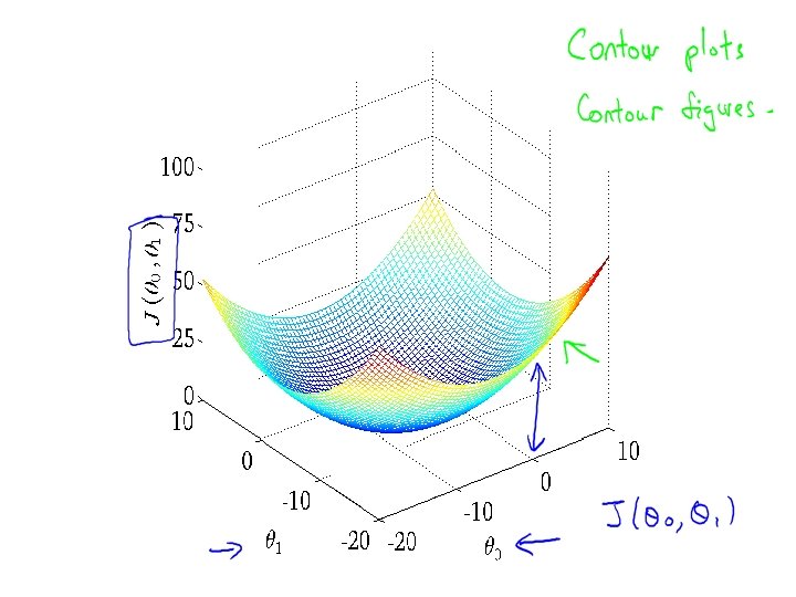
 1 0") J( 0, 1) 1 0
J( 0, 1) 1 0
 1 0") J( 0, 1) 1 0
J( 0, 1) 1 0
 Gradient descent algorithm Correct: Simultaneous update Incorrect:

 Linear regression with one variable Gradient descent intuition Machine Learning
 Gradient descent algorithm
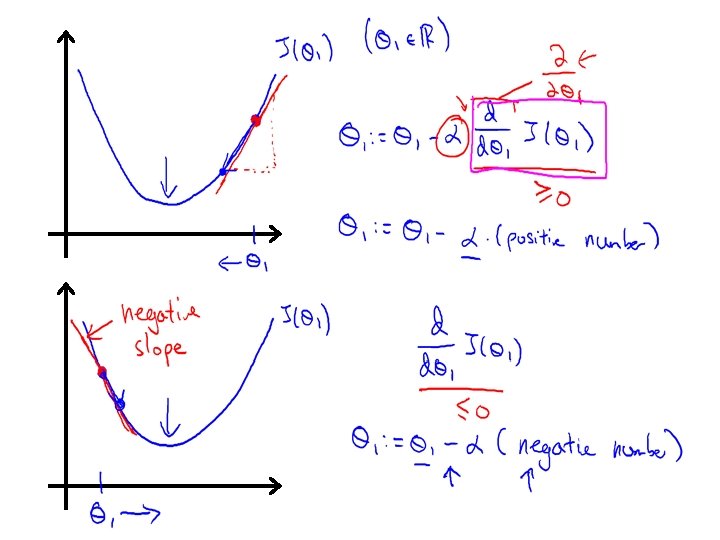
 If α is too small, gradient descent can be slow. If α is too large, gradient descent can overshoot the minimum. It may fail to converge, or even diverge.
 at local optima Current value of
 Gradient descent can converge to a local minimum, even with the learning rate α fixed. As we approach a local minimum, gradient descent will automatically take smaller steps. So, no need to decrease α over time.

 Linear regression with one variable Gradient descent for linear regression Machine Learning
 Gradient descent algorithm Linear Regression Model
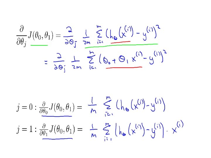
 Gradient descent algorithm update and simultaneously
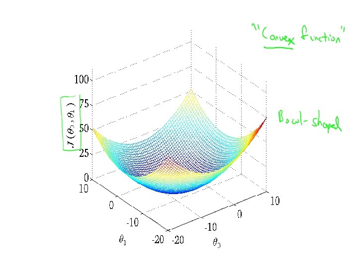
 1 0") J( 0, 1) 1 0
J( 0, 1) 1 0
 (function of the parameters )") (for fixed , this is a function of x) (function of the parameters )
(for fixed , this is a function of x) (function of the parameters )
 (function of the parameters )") (for fixed , this is a function of x) (function of the parameters )
(for fixed , this is a function of x) (function of the parameters )
 (function of the parameters )") (for fixed , this is a function of x) (function of the parameters )
(for fixed , this is a function of x) (function of the parameters )
 (function of the parameters )") (for fixed , this is a function of x) (function of the parameters )
(for fixed , this is a function of x) (function of the parameters )
 (function of the parameters )") (for fixed , this is a function of x) (function of the parameters )
(for fixed , this is a function of x) (function of the parameters )
 (function of the parameters )") (for fixed , this is a function of x) (function of the parameters )
(for fixed , this is a function of x) (function of the parameters )
 (function of the parameters )") (for fixed , this is a function of x) (function of the parameters )
(for fixed , this is a function of x) (function of the parameters )
 (function of the parameters )") (for fixed , this is a function of x) (function of the parameters )
(for fixed , this is a function of x) (function of the parameters )
 (function of the parameters )") (for fixed , this is a function of x) (function of the parameters )
(for fixed , this is a function of x) (function of the parameters )
 “Batch” Gradient Descent “Batch”: Each step of gradient descent uses all the training examples.

 Linear Regression with multiple variables Multiple features Machine Learning
. Size (feet 2) Price ($1000) 2104 1416 1534 852 … 460") Multiple features (variables). Size (feet 2) Price ($1000) 2104 1416 1534 852 … 460 232 315 178 …
Multiple features (variables). Size (feet 2) Price ($1000) 2104 1416 1534 852 … 460 232 315 178 …
. Number Size of (feet 2) bedroo Number ms of floors 2104") Multiple features (variables). Number Size of (feet 2) bedroo Number ms of floors 2104 1416 1534 852 Notation: … 5 3 3 2 … 1 2 2 1 … Age of home (years) Price ($1000) 45 40 30 36 … 460 232 315 178 … = number of features = input (features) of training example. = value of feature in training example.
Multiple features (variables). Number Size of (feet 2) bedroo Number ms of floors 2104 1416 1534 852 Notation: … 5 3 3 2 … 1 2 2 1 … Age of home (years) Price ($1000) 45 40 30 36 … 460 232 315 178 … = number of features = input (features) of training example. = value of feature in training example.
 Hypothesis: Previously:
 For convenience of notation, define . Multivariate linear regression.

 Linear Regression with multiple variables Gradient descent for multiple variables Machine Learning
") Hypothesis: Parameters: Cost function: Gradient descent: Repea t (simultaneously update for every )
Hypothesis: Parameters: Cost function: Gradient descent: Repea t (simultaneously update for every )
: Repeat (simultaneously update for ) (simultaneously") Gradient Descent New algorithm : Repeat Previously (n=1): Repeat (simultaneously update for ) (simultaneously update )
Gradient Descent New algorithm : Repeat Previously (n=1): Repeat (simultaneously update for ) (simultaneously update )

 Linear Regression with multiple variables Gradient descent in practice I: Feature Scaling Machine Learning
 Feature Scaling Idea: Make sure features are on a similar scale. E. g. = size (0 -2000 feet 2) = number of bedrooms (1 -5) size (feet 2) number of bedrooms
 Feature Scaling Get every feature into approximately a range.
 Mean normalization Replace with to make features have approximately zero mean (Do not apply to ). E. g.

 Linear Regression with multiple variables Gradient descent in practice II: Learning rate Machine Learning
 Gradient descent - “Debugging”: How to make sure gradient descent is working correctly. - How to choose learning rate .
 Making sure gradient descent is working correctly. Example automatic convergence test: Declare convergence if decreases by less than in one iteration. 0 100 200 300 No. of iterations 400
 Making sure gradient descent is working correctly. Gradient descent not working. Use smaller . No. of iterations - For sufficiently small , should decrease on every iteration. - But if is too small, gradient descent can be slow to converge.
 Summary: - If is too small: slow convergence. - If is too large: may not decrease on every iteration; may not converge. To choose , try

 Linear Regression with multiple variables Features and polynomial regression Machine Learning
 Housing prices prediction
 Size (x)") Polynomial regression Price (y) Size (x)
Polynomial regression Price (y) Size (x)
 Size (x)") Choice of features Price (y) Size (x)
Choice of features Price (y) Size (x)

 Linear Regression with multiple variables Normal equation Machine Learning
 Gradient Descent Normal equation: Method to solve for analytically.
 Solve for") Intuition: If 1 D (for every ) Solve for
Intuition: If 1 D (for every ) Solve for
 bedroo Number ms of floors 1 1 2104") Examples: Number Size of (feet 2) bedroo Number ms of floors 1 1 2104 1416 1534 852 5 3 3 2 1 2 2 1 Age of home (years) Price ($1000) 45 40 30 36 460 232 315 178
Examples: Number Size of (feet 2) bedroo Number ms of floors 1 1 2104 1416 1534 852 5 3 3 2 1 2 2 1 Age of home (years) Price ($1000) 45 40 30 36 460 232 315 178
 examples features. E. g. If ;
*X’*y") is inverse of matrix . Octave: pinv(X’*X)*X’*y
is inverse of matrix . Octave: pinv(X’*X)*X’*y
 training examples, features. Gradient Descent Normal Equation • Need to choose . • Needs many iterations. • Works well even when is large. • No need to choose . • Don’t need to iterate. • Need to compute • Slow if is very large.

") Linear Regression with multiple variables Machine Learning Normal equation and noninvertibility (optional)
Linear Regression with multiple variables Machine Learning Normal equation and noninvertibility (optional)
 - Octave: pinv(X’*X)*X’*y") Normal equation - What if is non-invertible? (singular/ degenerate) - Octave: pinv(X’*X)*X’*y
Normal equation - What if is non-invertible? (singular/ degenerate) - Octave: pinv(X’*X)*X’*y
. E. g. size in feet") What if is non-invertible? • Redundant features (linearly dependent). E. g. size in feet 2 size in m 2 • Too many features (e. g. ). - Delete some features, or use regularization.
What if is non-invertible? • Redundant features (linearly dependent). E. g. size in feet 2 size in m 2 • Too many features (e. g. ). - Delete some features, or use regularization.

 Linear model • Regression Function
 Linear model contd… Using matrix notation Where A is a m*n matrix
 Due to noise a small amount of error is added
 Least Square Estimator •
 Problem on Least Square Estimator
 Derivative Based Optimization • Deals with gradient-based optimization techniques, capable of determining search directions according to an objective function’s derivative information • Used in optimizing non-linear neuro-fuzzy models, – Steepest descent – Conjugate gradient
 = F ( x* + D x)") First-Order Optimality Condition T F ( x) = F ( x* + D x) = F ( x* ) + Ñ F ( x) For small Dx: If 1 T D x + -- D x Ñ 2 F ( x) Dx + ¼ * * 2 x=x If x* is a minimum, this implies: then But this would imply that x* is not a minimum. Therefore Since this must be true for every Dx,
First-Order Optimality Condition T F ( x) = F ( x* + D x) = F ( x* ) + Ñ F ( x) For small Dx: If 1 T D x + -- D x Ñ 2 F ( x) Dx + ¼ * * 2 x=x If x* is a minimum, this implies: then But this would imply that x* is not a minimum. Therefore Since this must be true for every Dx,
, then A strong minimum") Second-Order Condition If the first-order condition is satisfied (zero gradient), then A strong minimum will exist at x* if for any Dx ° 0. Therefore the Hessian matrix must be positive definite. A matrix A is positive definite if: for any z ° 0. This is a sufficient condition for optimality. A necessary condition is that the Hessian matrix be positive semidefinite. A matrix A is positive semidefinite if: for any z.
Second-Order Condition If the first-order condition is satisfied (zero gradient), then A strong minimum will exist at x* if for any Dx ° 0. Therefore the Hessian matrix must be positive definite. A matrix A is positive definite if: for any z ° 0. This is a sufficient condition for optimality. A necessary condition is that the Hessian matrix be positive semidefinite. A matrix A is positive semidefinite if: for any z.
 Basic Optimization Algorithm or pk - Search Direction ak - Learning Rate