Chapter 2 Data Mining Processes and Knowledge Discovery

Chapter 2 Data Mining Processes and Knowledge Discovery Identify actionable results

結束 Contents Describes the Cross-Industry Standard Process for Data Mining (CRISP-DM), a set of phases that can be used in data mining studies Discusses each phase in detail Gives an example illustration Discusses a knowledge discovery process 2 -2

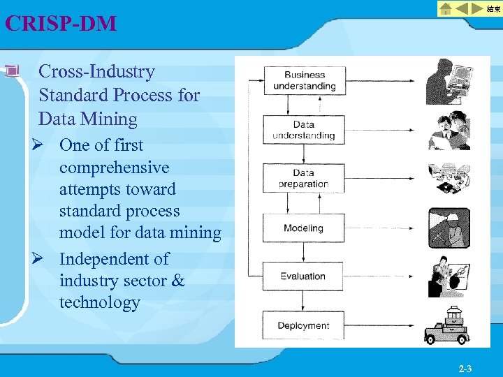結束 CRISP-DM Cross-Industry Standard Process for Data Mining Ø One of first comprehensive attempts toward standard process model for data mining Ø Independent of industry sector & technology 2 -3

結束 CRISP-DM Phases 1. Business (or problem) understanding 2. Data understanding Ø A systematic process to try to make sense of the massive amounts of data generated from daily operations. 3. Data preparation • Transform & create data set for modeling 4. Modeling 5. Evaluation • Check good models, evaluate to assure nothing missing 6. Deployment 2 -4

結束 Business Understanding Solve a specific problem Ø Determining business objectives, assessing the current situation, establishing data mining goals, and developing a project plan. Clear definition helps Ø Measurable success criteria Convert business objectives to set of data-mining goals Ø What to achieve in technical terms, such as üWhat types of customers are interested in each of our products? üWhat are typical profiles of customers … 2 -5

結束 Data Understanding Initial data collection, data description, data exploration, and the verification of data quality. Three issues considered in data selection: 1. Set up a concise and clear description of the problem. For example, a retail DM project may seek to identify spending behaviors of female shoppers who purchase seasonal clothes. 2. Identify the relevant data for the problem description, such demographical, credit card transactional, financial data… 3. Select variables for the relevant important for the project. 2 -6

結束 Data Understanding (cont. ) Data types: Ø Demographic data (income, education, age …) Ø Socio-graphic data (hobby, club membership, …) Ø Transactional data (sales record, credit card spending…) Ø Quantitative data: are measurable using numerical values) Ø Qualitative data: known as categorical data, contains both nominal and ordinal data. (see also page. 22) Related data: Can come from many sources? Ø Internal ü ERP (or MIS) ü Data Warehouse Ø External ü Government data ü Commercial data Ø Created ü Research 2 -7

結束 Data Preparation Once data sources available are identified, the data need to be selected, cleaned, built into the desired and formatted forms. Clean data: Formats, gaps, filters outliers & redundancies (see page. 22) Ø Unified numerical scales Ø Nominal data üCode (such gender data, male and female) Ø Ordinal data üNominal code or scale (excellent, fair, poor) Ø Cardinal data (Categorical, A, B, C levels) 2 -8

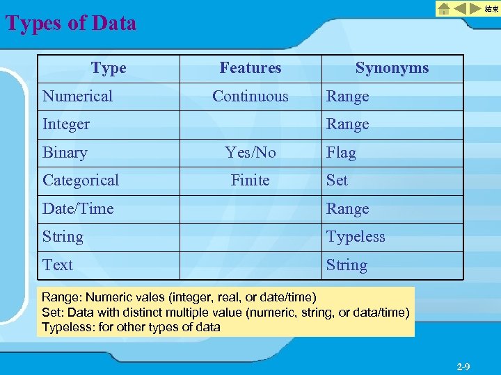結束 Types of Data Type Numerical Features Continuous Integer Binary Categorical Synonyms Range Yes/No Flag Finite Set Date/Time Range String Typeless Text String Range: Numeric vales (integer, real, or date/time) Set: Data with distinct multiple value (numeric, string, or data/time) Typeless: for other types of data 2 -9

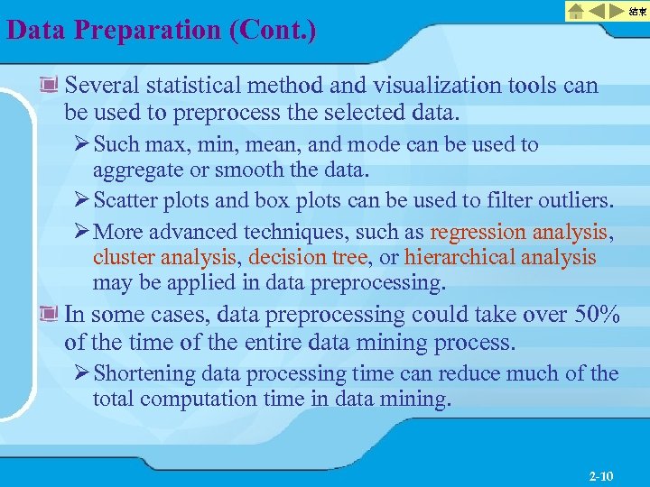結束 Data Preparation (Cont. ) Several statistical method and visualization tools can be used to preprocess the selected data. Ø Such max, min, mean, and mode can be used to aggregate or smooth the data. Ø Scatter plots and box plots can be used to filter outliers. Ø More advanced techniques, such as regression analysis, cluster analysis, decision tree, or hierarchical analysis may be applied in data preprocessing. In some cases, data preprocessing could take over 50% of the time of the entire data mining process. Ø Shortening data processing time can reduce much of the total computation time in data mining. 2 -10

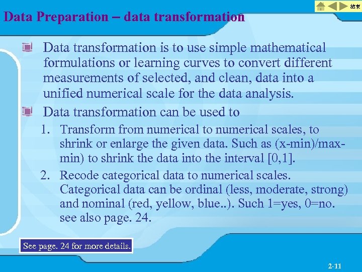結束 Data Preparation – data transformation Data transformation is to use simple mathematical formulations or learning curves to convert different measurements of selected, and clean, data into a unified numerical scale for the data analysis. Data transformation can be used to 1. Transform from numerical to numerical scales, to shrink or enlarge the given data. Such as (x-min)/maxmin) to shrink the data into the interval [0, 1]. 2. Recode categorical data to numerical scales. Categorical data can be ordinal (less, moderate, strong) and nominal (red, yellow, blue. . ). Such 1=yes, 0=no. see also page. 24. See page. 24 for more details. 2 -11

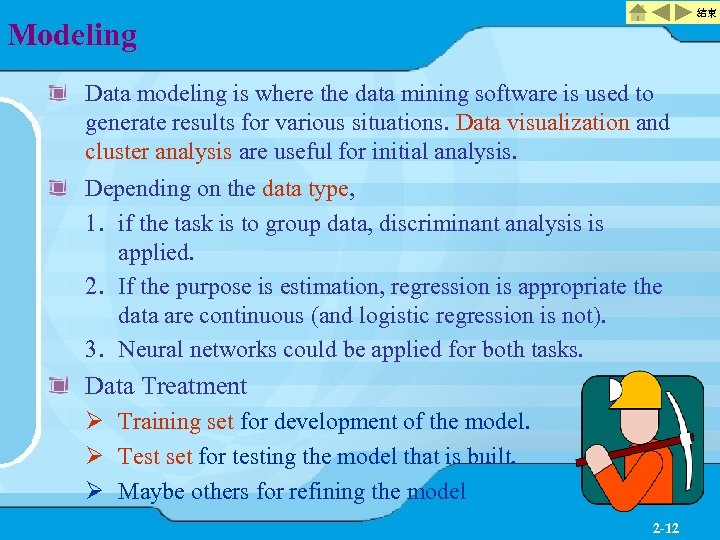結束 Modeling Data modeling is where the data mining software is used to generate results for various situations. Data visualization and cluster analysis are useful for initial analysis. Depending on the data type, 1. if the task is to group data, discriminant analysis is applied. 2. If the purpose is estimation, regression is appropriate the data are continuous (and logistic regression is not). 3. Neural networks could be applied for both tasks. Data Treatment Ø Training set for development of the model. Ø Test set for testing the model that is built. Ø Maybe others for refining the model 2 -12

結束 Data mining techniques Techniques Ø Association: the relationship of a particular item in a data transaction on other items in the same transaction is used to predict patterns. See also page 25 for example. Ø Classification: the methods are intended for learning different functions that map each item of the selected data into one of a predefined set of classes. Two key research problems related to classification results are the evaluation of misclassification and prediction power(C 4. 5). üMathematical modeling is often used to construct classification methods are binary decision trees (CART), neural networks (nonlinear), linear programming (boundary), and statistics. üSee also page. 25, 26 for more explanations 2 -13

結束 Data mining techniques (Cont. ) Ø Clustering: taking ungrouped data and uses automatic techniques to put this data into groups. üClustering is unsupervised and does not require a learning set. (Chapter 5) Ø Predictions: is related to regression technique, to discover the relationship between the dependent and independent variables. Ø Sequential patterns: seeks to find similar patterns in data transaction over a business period. üThe mathematical models behind sequential patterns are logic rules, fuzzy logic, and so on. üSimilar time sequences: applied to discover sequences similar to a known sequence over both past and current business periods. 2 -14

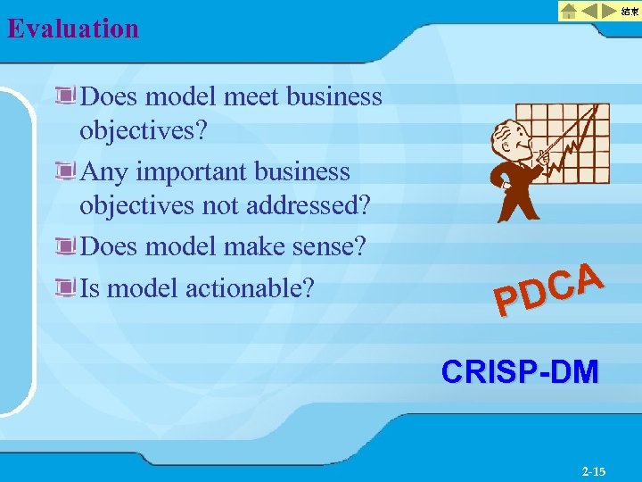結束 Evaluation Does model meet business objectives? Any important business objectives not addressed? Does model make sense? Is model actionable? CA PD CRISP-DM 2 -15

結束 Deployment DM can be used to verify previously held hypotheses or for knowledge discovery. DM models can be applied to business purposes , including prediction or identification of key situations Ongoing monitoring & maintenance Ø Evaluate performance against success criteria Ø Market reaction & competitor changes (remodeling or fine tune) 2 -16

結束 Example Training set for computer purchase Ø 16 records Ø 5 attributes Goal ØFind classifier for consumer behavior 2 -17

結束 Database (1 st half) Case Age Income Student Credit Gender Buy? A 1 31 -40 High No Fair Male Yes A 2 >40 Medium No Fair Female Yes A 3 >40 Low Yes Fair Female Yes A 4 31 -40 Low Yes Excellent Female Yes A 5 ≤ 30 Low Yes Fair Female Yes A 6 >40 Medium Yes Fair Male Yes A 7 ≤ 30 Medium Yes Excellent Male Yes A 8 31 -40 Medium No Excellent Male Yes 2 -18

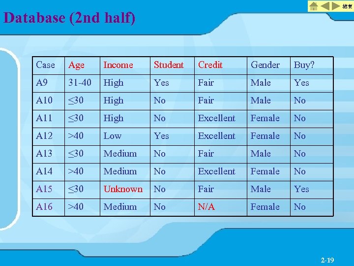結束 Database (2 nd half) Case Age Income Student Credit Gender Buy? A 9 31 -40 High Yes Fair Male Yes A 10 ≤ 30 High No Fair Male No A 11 ≤ 30 High No Excellent Female No A 12 >40 Low Yes Excellent Female No A 13 ≤ 30 Medium No Fair Male No A 14 >40 Medium No Excellent Female No A 15 ≤ 30 Unknown No Fair Male Yes A 16 >40 Medium No N/A Female No 2 -19

結束 Data Selection Gender has weak relationship with purchase Ø Based on correlation Ø Drop gender Selected Attribute Set {Age, Income, Student, Credit} 2 -20

結束 Data Preprocessing Income unknown in Case 15 Credit not available in Case 16 Drop these noisy cases 2 -21

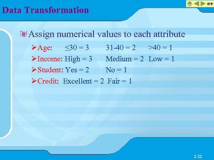結束 Data Transformation Assign numerical values to each attribute Ø Age: ≤ 30 = 3 31 -40 = 2 >40 = 1 Ø Income: High = 3 Medium = 2 Low = 1 Ø Student: Yes = 2 No = 1 Ø Credit: Excellent = 2 Fair = 1 2 -22

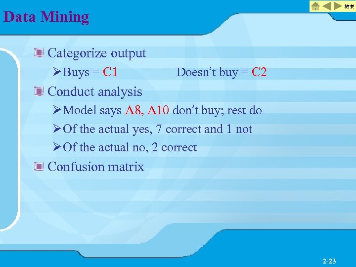結束 Data Mining Categorize output Ø Buys = C 1 Doesn’t buy = C 2 Conduct analysis Ø Model says A 8, A 10 don’t buy; rest do Ø Of the actual yes, 7 correct and 1 not Ø Of the actual no, 2 correct Confusion matrix 2 -23

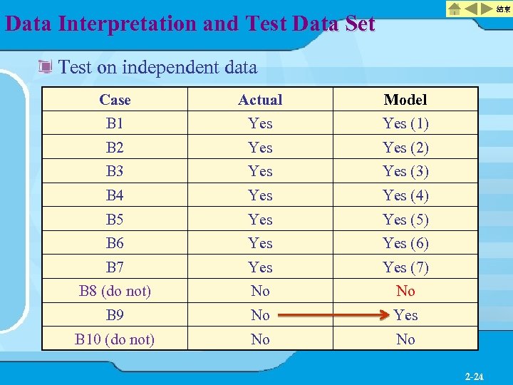結束 Data Interpretation and Test Data Set Test on independent data Case Actual Model B 1 Yes (1) B 2 Yes (2) B 3 Yes (3) B 4 Yes (4) B 5 Yes (5) B 6 Yes (6) B 7 Yes (7) B 8 (do not) No No B 9 No Yes B 10 (do not) No No 2 -24

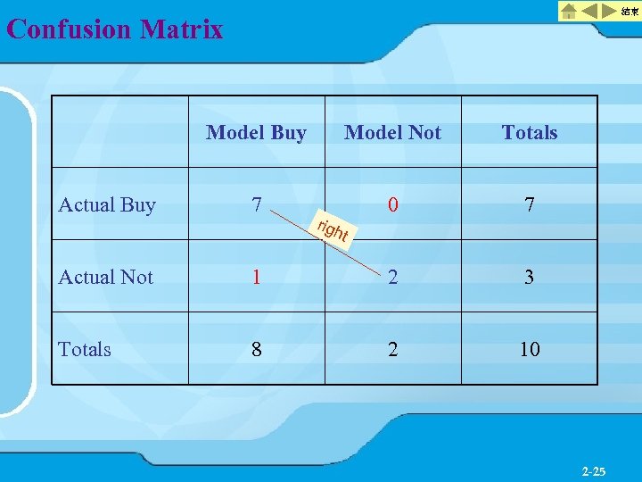結束 Confusion Matrix Model Buy Actual Buy Model Not Totals 7 0 7 righ t Actual Not 1 2 3 Totals 8 2 10 2 -25

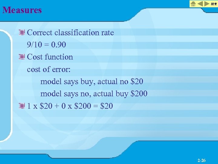結束 Measures Correct classification rate 9/10 = 0. 90 Cost function cost of error: model says buy, actual no $20 model says no, actual buy $200 1 x $20 + 0 x $200 = $20 2 -26

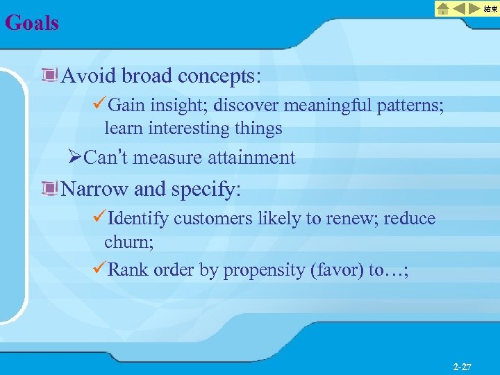結束 Goals Avoid broad concepts: üGain insight; discover meaningful patterns; learn interesting things ØCan’t measure attainment Narrow and specify: üIdentify customers likely to renew; reduce churn; üRank order by propensity (favor) to…; 2 -27

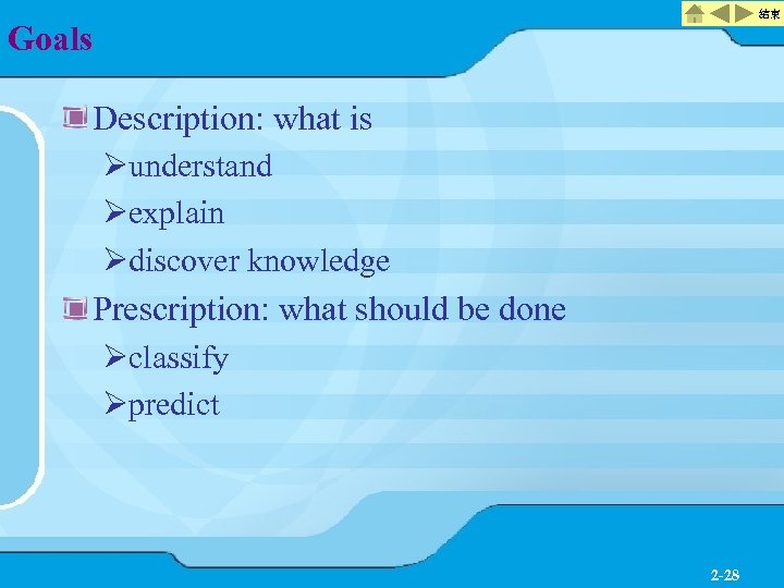結束 Goals Description: what is Øunderstand Øexplain Ødiscover knowledge Prescription: what should be done Øclassify Øpredict 2 -28

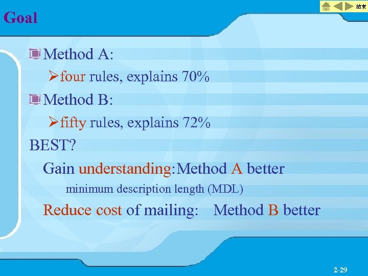結束 Goal Method A: Øfour rules, explains 70% Method B: Øfifty rules, explains 72% BEST? Gain understanding: Method A better minimum description length (MDL) Reduce cost of mailing: Method B better 2 -29

結束 Measurement Accuracy ØHow well does model describe observed data? Confidence levels Ø a proportion of the time between lower and upper limits Comprehensibility Whole or parts? 2 -30

結束 Measuring Predictive Classification & prediction: error rate = incorrect/total requires evaluation set be representative Estimators predicted - actual (MAD, MSE, MAPE) variance = sum(predicted - actual)^2 standard deviation = square root of variance distance - how far off 2 -31

結束 Statistics Population - entire group studied Sample - subset from population Bias - difference between sample average & population average Ømean, median, mode Ødistribution Øsignificance Øcorrelation, regression (hamming distance) 2 -32

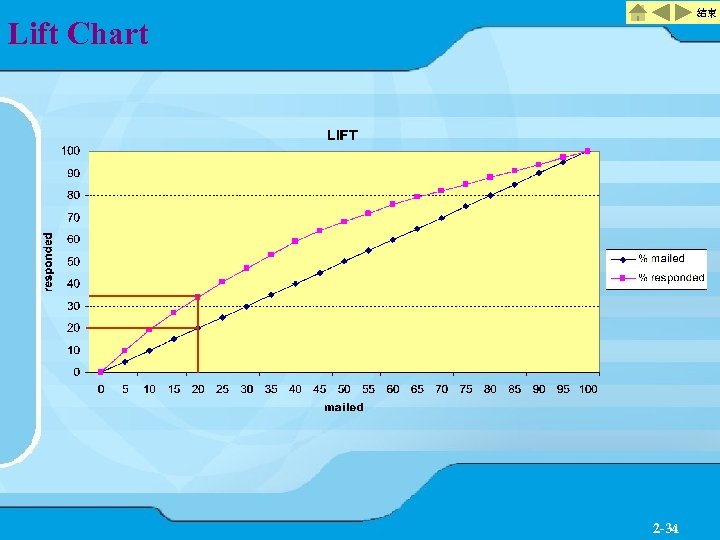
結束 Classification Models LIFT = probability in class by sample divided by probability in class by population Øif population probability is 20% and sample probability is 30%, LIFT = 0. 3/0. 2 = 1. 5 Best lift not necessarily best need sufficient sample size as confidence increase. 2 -33

結束 Lift Chart 2 -34

結束 Measuring Impact Ideal - $ (NPV) because of expenditure Mass mailing may be better Depends on: Ø fixed cost Ø cost per recipient Ø cost per respondent Ø value of positive response 2 -35

結束 Bottom Line Return on investment 2 -36

結束 Example Application Telephone industry Problem: Unpaid bills Data mining used to develop models to predict nonpayment as early as possible See page. 27 2 -37

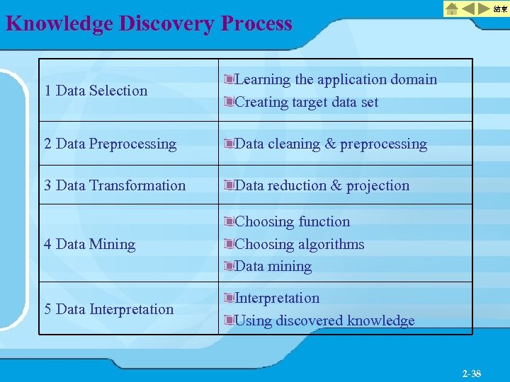結束 Knowledge Discovery Process 1 Data Selection Learning the application domain Creating target data set 2 Data Preprocessing Data cleaning & preprocessing 3 Data Transformation Data reduction & projection 4 Data Mining Choosing function Choosing algorithms Data mining 5 Data Interpretation Using discovered knowledge 2 -38

結束 1: Business Understanding Predict which customers would be insolvent ØIn time for firm to take preventive measures (and avert losing good customers) Hypothesis: ØInsolvent customers would change calling habits & phone usage during a critical period before & immediately after termination of billing period 2 -39

結束 2: Data Understanding Static customer information available in files ØBills, payments, usage Used data warehouse to gather & organize data ØCoded to protect customer privacy 2 -40

結束 Creating Target Data Set Customer files ØCustomer information ØDisconnects ØReconnections Time-dependent data ØBills ØPayments ØUsage 100, 000 customers over 17 -month period Stratified (hierarchical) sampling to assure all groups appropriately represented 2 -41

結束 3: Data Preparation Filtered out incomplete data Deleted inexpensive calls Ø Reduced data volume about 50% Low number of fraudulent cases Cross-checked with phone disconnects Lagged data made synchronization necessary 2 -42

結束 Data Reduction & Projection Information grouped by account Customer data aggregated by 2 -week periods Discriminant analysis on 23 categories Calculated average owed by category (significant) Identified extra charges (significant) Investigated payment by installments (not significant) 2 -43

結束 Choosing Data Mining Function Classes: Ø Most possibly solvent (99. 3%) Ø Most possibly insolvent (0. 7%) Costs of error widely different New data set created through stratified sampling Ø Retained all insolvent Ø Altered distribution to 90% solvent Ø Used 2, 066 cases total Critical period identified Ø Last 15 two-week periods before service interruption Variables defined by counting measures in twoweek periods Ø 46 variables as candidate discriminant factors 2 -44

結束 4: Modeling Discriminant Analysis Ø Linear model Ø SPSS – stepwise forward selection Decision Trees Ø Rule-based classifier, C 5, C 4. 5 Neural Networks Ø Nonlinear model 2 -45

結束 Data Mining Training set about 2/3 rds Rest test Discriminant analysis Ø Used 17 variables Ø Equal costs – 0. 875 correct Ø Unequal costs – 0. 930 correct Rule-based – 0. 952 correct Neural network – 0. 929 correct 2 -46

結束 5: Evaluation 1 st objective to maximize accuracy of predicting insolvent customers Ø Decision tree classifier best 2 nd objective to minimize error rate for solvent customers Ø Neural network model close to Decision tree Used all 3 on case-by-case basis 2 -47

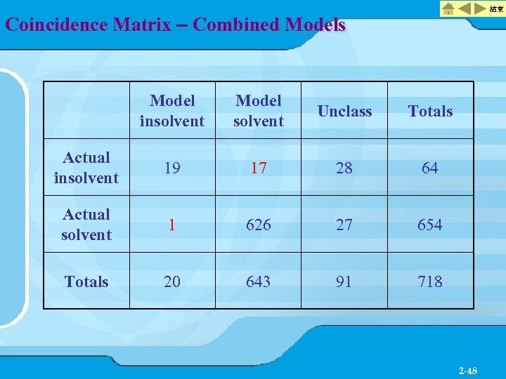結束 Coincidence Matrix – Combined Models Model insolvent Model solvent Unclass Totals Actual insolvent 19 17 28 64 Actual solvent 1 626 27 654 Totals 20 643 91 718 2 -48

結束 6: Implementation Every customer examined using all 3 algorithms ØIf all 3 agreed, used that classification ØIf disagreement, categorized as unclassified Correct on test data 0. 898 ØOnly 1 actually solvent customer would have been disconnected 2 -49