Chapter 19 Financing and Valuation Recall that

Chapter 19 Financing and Valuation • Recall that there are three questions in corporate finance. • The first regards what long-term investments the firm should make (the capital budgeting question). • The second regards the use of debt (the capital structure question). • This chapter is the nexus of these questions. 1

The 3 Methods for Valuation 1. After Tax WACC 2. Flow of Equity Method 3. Adjusted Present Value 2

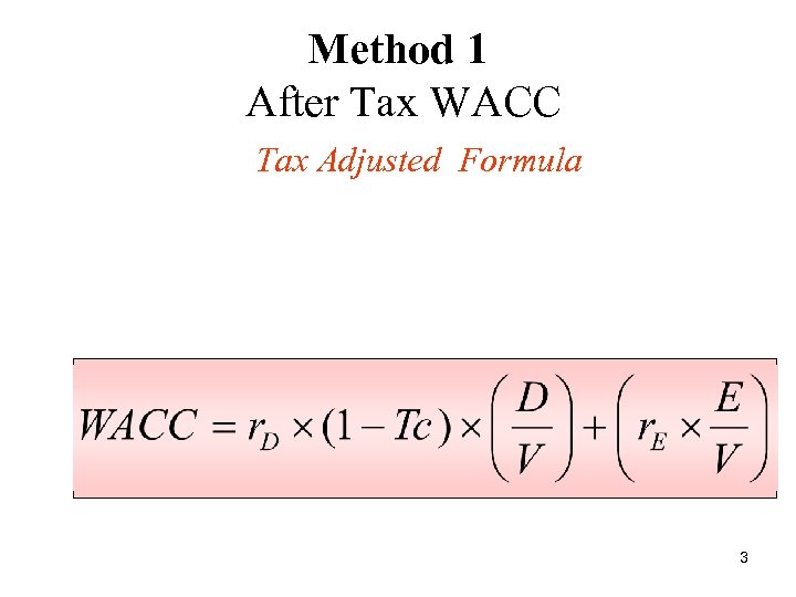Method 1 After Tax WACC Tax Adjusted Formula 3

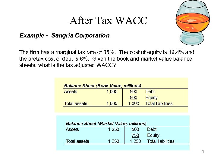After Tax WACC Example - Sangria Corporation The firm has a marginal tax rate of 35%. The cost of equity is 12. 4% and the pretax cost of debt is 6%. Given the book and market value balance sheets, what is the tax adjusted WACC? 4

After Tax WACC Example - Sangria Corporation - continued The company would like to invest in a perpetual crushing machine with cash flows of $1. 731 million per year pre-tax. Given an initial investment of $12. 5 million, what is the value of the machine? 5

Remember with WACC Approach ! • Since tax shield is accounted for in the cost of capital, calculate cash flows as if the company is all equity financed. • WACC approach values the assets and operations of the company. If you are interested in equity value, do not forget to subtract the value of the company’s debt. 6

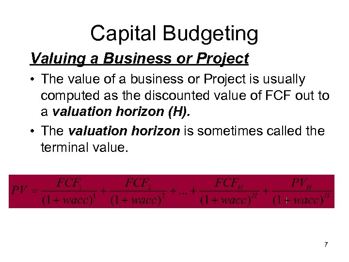Capital Budgeting Valuing a Business or Project • The value of a business or Project is usually computed as the discounted value of FCF out to a valuation horizon (H). • The valuation horizon is sometimes called the terminal value. 7

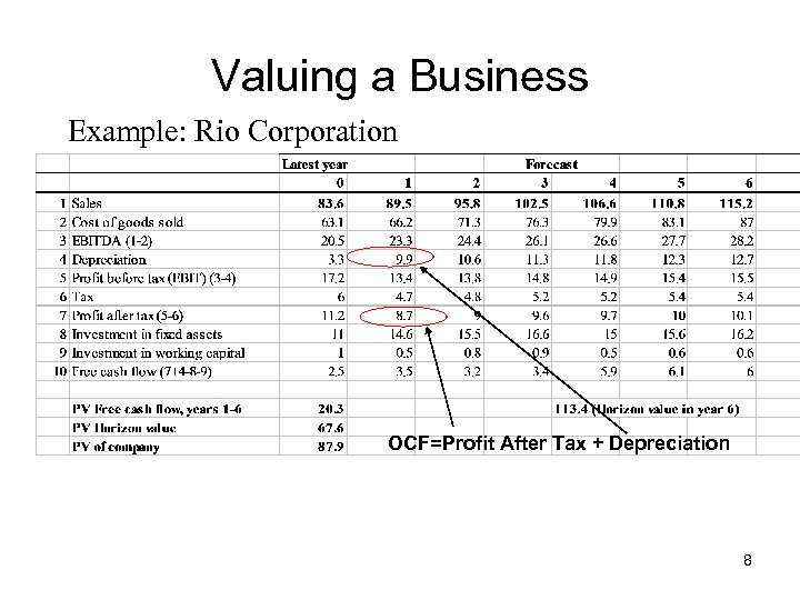Valuing a Business Example: Rio Corporation OCF=Profit After Tax + Depreciation 8

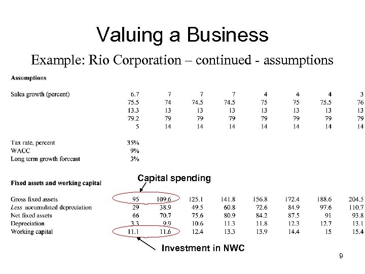Valuing a Business Example: Rio Corporation – continued - assumptions Capital spending Investment in NWC 9

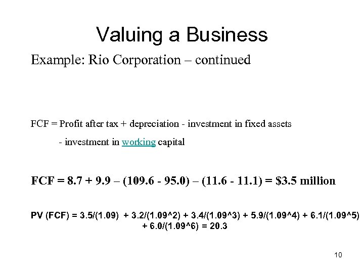Valuing a Business Example: Rio Corporation – continued FCF = Profit after tax + depreciation - investment in fixed assets - investment in working capital FCF = 8. 7 + 9. 9 – (109. 6 - 95. 0) – (11. 6 - 11. 1) = $3. 5 million PV (FCF) = 3. 5/(1. 09) + 3. 2/(1. 09^2) + 3. 4/(1. 09^3) + 5. 9/(1. 09^4) + 6. 1/(1. 09^5) + 6. 0/(1. 09^6) = 20. 3 10

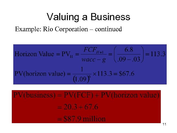Valuing a Business Example: Rio Corporation – continued 11

Things to Consider 1. Don’t value mechanically – for terminal value it might be wise to use knowledge about mature firms in the industry. 2. Liquidation value. 12

In Practice How are costs of financing determined? – – – What is included in debt? What if there are other securities? How do we determine debt return? How do we determine preferred stock return? What if project has a different leverage ratio? How do we determine equity return for a firm that is not yet traded, or (and) had a different leverage than what we observe in the stock market? 13

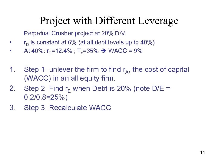Project with Different Leverage • • 1. 2. 3. Perpetual Crusher project at 20% D/V r. D is constant at 6% (at all debt levels up to 40%) At 40%: r. E=12. 4% ; Tc=35% WACC = 9% Step 1: unlever the firm to find r. A, the cost of capital (WACC) in an all equity firm. Step 2: Find r. E when Debt is 20% (note D/E = 0. 2/0. 8=25%) Step 3: Recalculate WACC 14

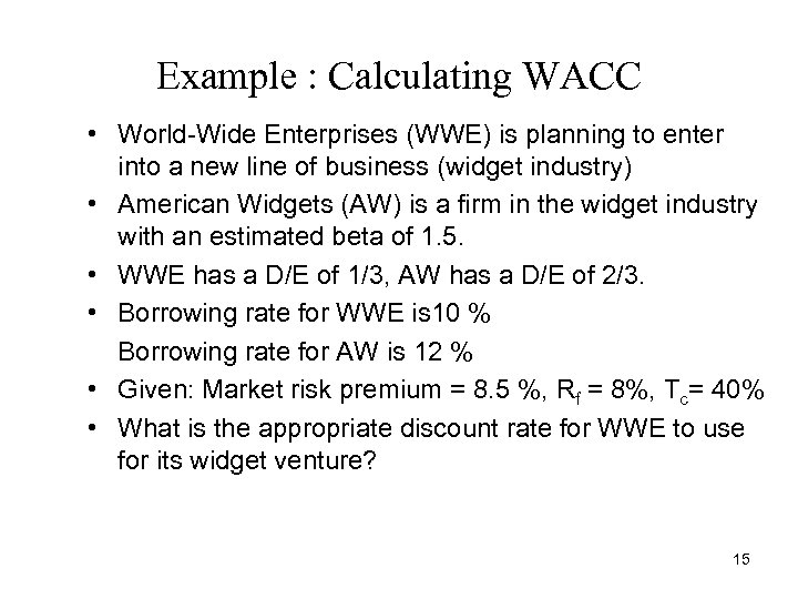Example : Calculating WACC • World-Wide Enterprises (WWE) is planning to enter into a new line of business (widget industry) • American Widgets (AW) is a firm in the widget industry with an estimated beta of 1. 5. • WWE has a D/E of 1/3, AW has a D/E of 2/3. • Borrowing rate for WWE is 10 % Borrowing rate for AW is 12 % • Given: Market risk premium = 8. 5 %, Rf = 8%, Tc= 40% • What is the appropriate discount rate for WWE to use for its widget venture? 15

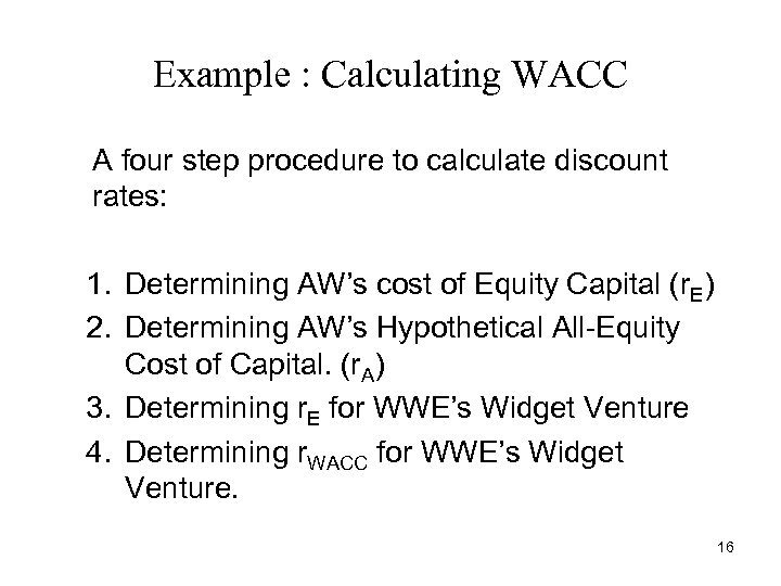Example : Calculating WACC A four step procedure to calculate discount rates: 1. Determining AW’s cost of Equity Capital (r. E) 2. Determining AW’s Hypothetical All-Equity Cost of Capital. (r. A) 3. Determining r. E for WWE’s Widget Venture 4. Determining r. WACC for WWE’s Widget Venture. 16

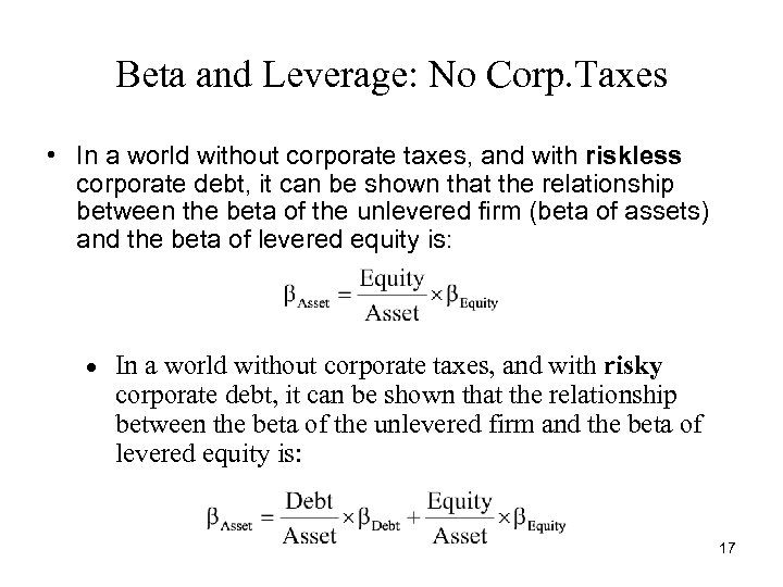Beta and Leverage: No Corp. Taxes • In a world without corporate taxes, and with riskless corporate debt, it can be shown that the relationship between the beta of the unlevered firm (beta of assets) and the beta of levered equity is: · In a world without corporate taxes, and with risky corporate debt, it can be shown that the relationship between the beta of the unlevered firm and the beta of levered equity is: 17

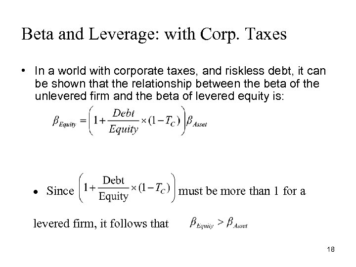Beta and Leverage: with Corp. Taxes • In a world with corporate taxes, and riskless debt, it can be shown that the relationship between the beta of the unlevered firm and the beta of levered equity is: · Since must be more than 1 for a levered firm, it follows that 18

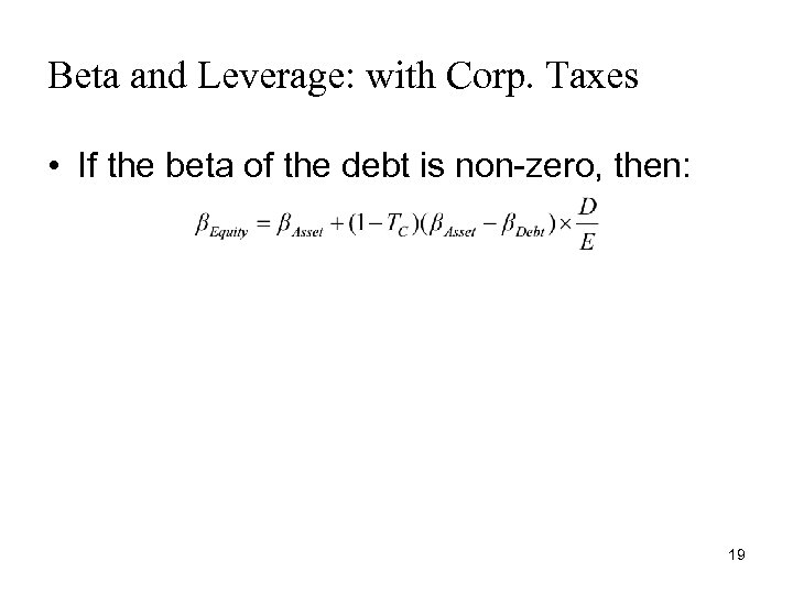Beta and Leverage: with Corp. Taxes • If the beta of the debt is non-zero, then: 19

Method 2 Flow to Equity Approach • Discount the cash flow from the project to the equity holders of the levered firm at the cost of levered equity capital, r. E. • There are three steps in the FTE Approach: – Step One: Calculate the levered cash flows – Step Two: Calculate r. E. – Step Three: Valuation of the levered cash flows at r. E. 20

Flow to Equity Sangria Corporation - continued The company would like to invest in a perpetual crushing machine with cash flows of $1. 731 million per year pre-tax. Given an initial investment of $12. 5 million, what is the value of the machine? Remember: r. E = 12. 4%, D=$5 million (40% of project’s cost), r. D = 6%, TC=35%. 21

Method 2 Adjusted Present Value APV = Base Case NPV+ PV Impact 1. Base Case = All equity finance NPV – Discount unlevered cashflow by unlevered cost of equity (r. A), assuming not tax world. 2. PV Impact = all costs/benefits directly resulting from project - Discount all cost/benefits of financing according to their particular risk. 22

Adjusted Present Value Sangria Corporation - continued The company would like to invest in a perpetual crushing machine with cash flows of $1. 731 million per year pre-tax. Given an initial investment of $12. 5 million, what is the value of the machine? Remember: r. E = 12. 4%, D=$5 million (40% of project’s cost), r. D = 6%, TC=35%. 23

Side Effects in APV – Easy to Add Up Example: Project A has an NPV of $150, 000. In order to finance the project we must issue stock, with a brokerage cost of $200, 000. Project B has a NPV of -$20, 000. We can issue debt at 8% to finance the project. The new debt has a PV Tax Shield of $60, 000.

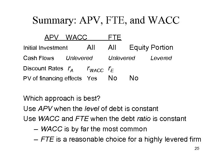Summary: APV, FTE, and WACC APV WACC Initial Investment All FTE All Cash Flows Unlevered r. WACC r. E PV of financing effects Yes No Discount Rates Equity Portion Levered r. A No Which approach is best? Use APV when the level of debt is constant Use WACC and FTE when the debt ratio is constant – WACC is by far the most common – FTE is a reasonable choice for a highly levered firm 25

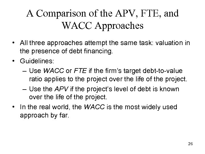A Comparison of the APV, FTE, and WACC Approaches • All three approaches attempt the same task: valuation in the presence of debt financing. • Guidelines: – Use WACC or FTE if the firm’s target debt-to-value ratio applies to the project over the life of the project. – Use the APV if the project’s level of debt is known over the life of the project. • In the real world, the WACC is the most widely used approach by far. 26

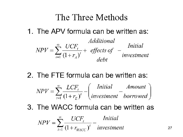The Three Methods 1. The APV formula can be written as: 2. The FTE formula can be written as: 3. The WACC formula can be written as 27

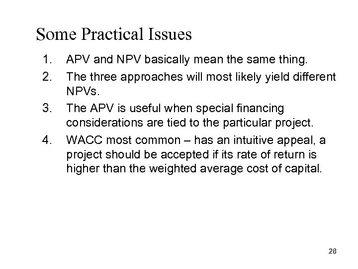Some Practical Issues 1. 2. 3. 4. APV and NPV basically mean the same thing. The three approaches will most likely yield different NPVs. The APV is useful when special financing considerations are tied to the particular project. WACC most common – has an intuitive appeal, a project should be accepted if its rate of return is higher than the weighted average cost of capital. 28

WACC Approach WACC approach is the most widely used because of its relative simplicity. WACC is only appropriate as a discount rate for a project when: 1. The project has similar systematic business risk as the firm. 2. The project and firm have the same debt capacity. 3. The debt to equity ratio is presumed to stay constant throughout the life of the project. 29

Discounting Safe Cash Flows (for APV Approach) Safe (risk-free) cash flows are discounted by the after tax borrowing rate r. D(1 -TC). This may be applied for issues such as subsidized loans and depreciation tax shields. Example: The company is granted a one-year subsidized loan of $100 k at 5%. The company’s borrowing rate is 13% and its tax rate 35%. What is the NPV of the loan? 30

PMM’s Project Valuation - APV 1. 2. Suppose PMM Inc. has an investment that costs $10, 000 with expected EBIT (cash flows from operations) of $3, 030, 303 per year forever. The investment can be financed either with $10, 000 in equity or with $5, 000 of 10% debt and $5, 000 of internally generated (equity) cash flows. The discount rate on an all‑equity-financed project with this kind of risk is 20%. The firm's marginal tax rate is 34%. Using the APV approach – find whether the project should be pursued if financed with equity only. Using the APV approach – find whether the project should be pursued if financed with 50% debt. 31

PMM’s Project Valuation with Subsidy Extension 1 : Subsidized (or below‑market‑rate) financing Suppose a municipal government decides that the investment is socially (and politically) desirable and agrees to raise the $5, 000 debt financing as a municipal bond, or 'muni. ' PPM Inc. can effectively borrow $5, 000 at the municipality's borrowing rate, r. D = 7%. (Interest income on a muni is exempt from Federal tax, so the muni rate is typically below the rate on corporate debt. ) Using APV approach – find the effect of this subsidy on APV. 32

PMM’s Project Valuation with Subsidy Extension 2 : Flotation Costs When a company raises funds through external debt or equity, it must incur flotation costs. Assume that the municipal government no longer sponsored the project and PPM Inc. must obtain $5, 000 with new debt at the market interest rate of 10%. Flotation costs are 12. 5% of gross proceeds. Assume that the Canadian tax code allows this expense to be amortized over five years. Using APV approach – find the effect of flotation costs on APV. 33

PMM’s Project Valuation – Flow to Equity Suppose PMM Inc. has an investment that costs $10, 000 with expected EBIT (cash flows from operations) of $3, 030, 303 per year forever. The investment can be financed with $5, 000 of 10% debt and $5, 000 of internally generated (equity) cash flows. The discount rate on an all‑equity-financed project with this kind of risk is 20%. The firm's marginal tax rate is 34%. Assume D/E = 50/67. Using the Flow to equity approach find whether the project should be pursued if financed with 50% debt. 34

PMM’s Project Valuation – WACC Suppose PMM Inc. has an investment that costs $10, 000 with expected EBIT (cash flows from operations) of $3, 030, 303 per year forever. The investment can be financed with $5, 000 of 10% debt and $5, 000 of internally generated (equity) cash flows. The discount rate on an all‑equity-financed project with this kind of risk is 20%. The firm's marginal tax rate is 34%. Assume D/E = 50/67. Using the WACC approach find whether the project should be pursued if financed with 50% debt. 35

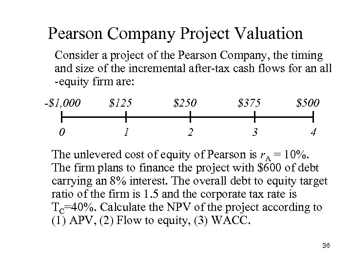Pearson Company Project Valuation Consider a project of the Pearson Company, the timing and size of the incremental after-tax cash flows for an all -equity firm are: -$1, 000 0 $125 $250 $375 $500 1 2 3 4 The unlevered cost of equity of Pearson is r. A = 10%. The firm plans to finance the project with $600 of debt carrying an 8% interest. The overall debt to equity target ratio of the firm is 1. 5 and the corporate tax rate is TC=40%. Calculate the NPV of the project according to (1) APV, (2) Flow to equity, (3) WACC. 36

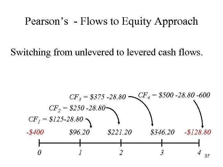Pearson’s - Flows to Equity Approach Switching from unlevered to levered cash flows. CF 3 = $375 -28. 80 CF 4 = $500 -28. 80 -600 CF 2 = $250 -28. 80 CF 1 = $125 -28. 80 -$400 0 $96. 20 $221. 20 $346. 20 -$128. 80 1 2 3 4 37

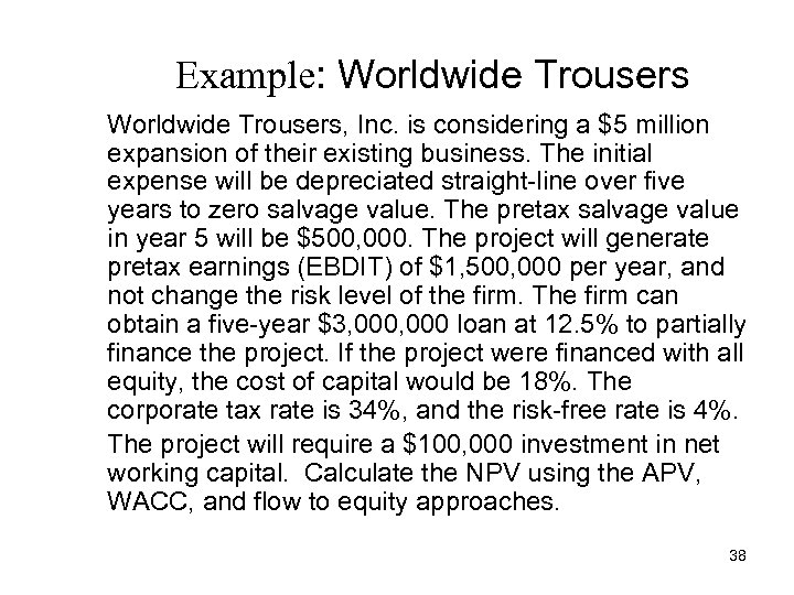Example: Worldwide Trousers, Inc. is considering a $5 million expansion of their existing business. The initial expense will be depreciated straight-line over five years to zero salvage value. The pretax salvage value in year 5 will be $500, 000. The project will generate pretax earnings (EBDIT) of $1, 500, 000 per year, and not change the risk level of the firm. The firm can obtain a five-year $3, 000 loan at 12. 5% to partially finance the project. If the project were financed with all equity, the cost of capital would be 18%. The corporate tax rate is 34%, and the risk-free rate is 4%. The project will require a $100, 000 investment in net working capital. Calculate the NPV using the APV, WACC, and flow to equity approaches. 38

Relative Valuation Valuing a company relative to another company 39

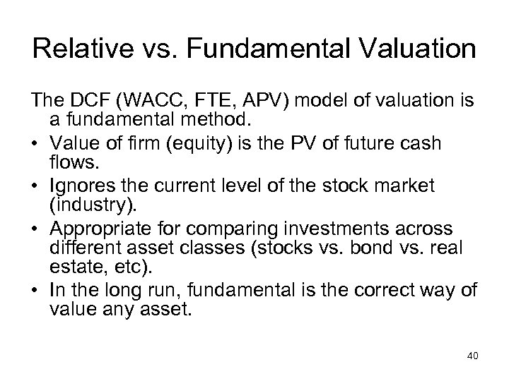Relative vs. Fundamental Valuation The DCF (WACC, FTE, APV) model of valuation is a fundamental method. • Value of firm (equity) is the PV of future cash flows. • Ignores the current level of the stock market (industry). • Appropriate for comparing investments across different asset classes (stocks vs. bond vs. real estate, etc). • In the long run, fundamental is the correct way of value any asset. 40

Relative vs. Fundamental Valuation Relative valuation is based on P/E ratios and a host of other “multiples”. • Extremely popular with the press, CNBS, Stock brokers • Used to value one stock against another. • Can not compare value across different asset classes (stocks vs. bond vs. real estate, etc). • Can not answer the question is the “stock market over valued? ” • Can answer the question, “I want to buy a tech stock, which one should I buy? ” • Can answer the question, “Which one of these overpriced IPO’s is the best buy? ” 41

Relative vs. Fundamental Valuation You are investing for your retirement. You are planning to take a buy and hold strategy which involves picking some fairly priced stocks and holding them for several years. Which valuation approach should you use? Relative or fundamental? 42

Relative vs. Fundamental Valuation You are a short term investor. You trade several times a week on your E-trade account, and rarely hold a stock for more than a month. Which valuation technique should you use? Relative or fundamental? 43

Relative Valuation Prices can be standardized using a common variable such as earnings, cashflows, book value, or revenues. Earnings Multiples • Price/Earning ratio (PE) and variants • Value/EBIT • Value/EBDITA • Value/Cashflow • Enterprise value/EBDITA Book Multiples • Price/Book Value (of equity) PBV Revenues • Price/Sales per Share (PS) • Enterprise Value/Sales per Share (EVS) Industry Specific Variables (Price/kwh, Price per ton of steel, Price per click, Price per labor hour) 44

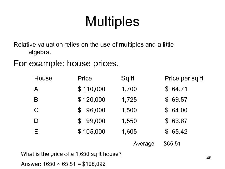Multiples Relative valuation relies on the use of multiples and a little algebra. For example: house prices. House Price Sq ft Price per sq ft A $ 110, 000 1, 700 $ 64. 71 B $ 120, 000 1, 725 $ 69. 57 C $ 96, 000 1, 500 $ 64. 00 D $ 99, 000 1, 550 $ 63. 87 E $ 105, 000 1, 605 $ 65. 42 Average $65. 51 What is the price of a 1, 650 sq ft house? Answer: 1650 × 65. 51 = $108, 092 45

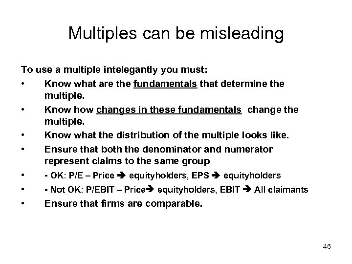Multiples can be misleading To use a multiple intelegantly you must: • Know what are the fundamentals that determine the multiple. • Know how changes in these fundamentals change the multiple. • Know what the distribution of the multiple looks like. • Ensure that both the denominator and numerator represent claims to the same group • - OK: P/E – Price equityholders, EPS equityholders • - Not OK: P/EBIT – Price equityholders, EBIT All claimants • Ensure that firms are comparable. 46

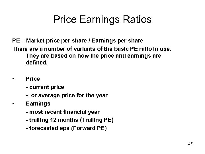Price Earnings Ratios PE – Market price per share / Earnings per share There a number of variants of the basic PE ratio in use. They are based on how the price and earnings are defined. • • Price - current price - or average price for the year Earnings - most recent financial year - trailing 12 months (Trailing PE) - forecasted eps (Forward PE) 47

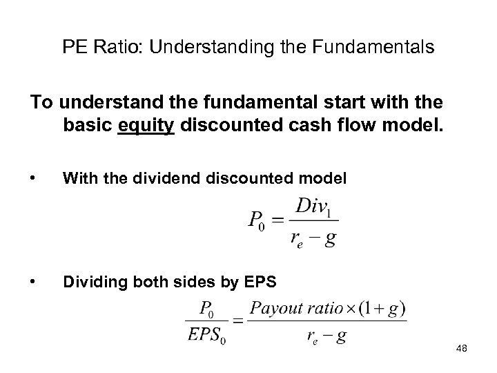PE Ratio: Understanding the Fundamentals To understand the fundamental start with the basic equity discounted cash flow model. • With the dividend discounted model • Dividing both sides by EPS 48

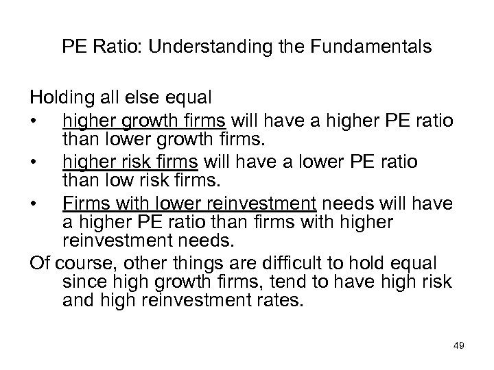PE Ratio: Understanding the Fundamentals Holding all else equal • higher growth firms will have a higher PE ratio than lower growth firms. • higher risk firms will have a lower PE ratio than low risk firms. • Firms with lower reinvestment needs will have a higher PE ratio than firms with higher reinvestment needs. Of course, other things are difficult to hold equal since high growth firms, tend to have high risk and high reinvestment rates. 49

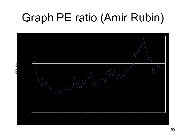Graph PE ratio (Amir Rubin) 50

Is low (high) PE cheap (expensive)? • A market strategist argues that stocks are over priced because the PE ratio today is too high relative to the average PE ratio across time. Do you agree? • Yes • No • If you do not agree, what factor might explain the high PE ratio today? 51

A Question You are reading an equity research report on Informix, and the analyst claims that the stock is undervalued because its PE ratio is 9. 71 while the average of the sector PE ratio is 35. 51. Would you agree? • Yes • No • Why or why not? 52

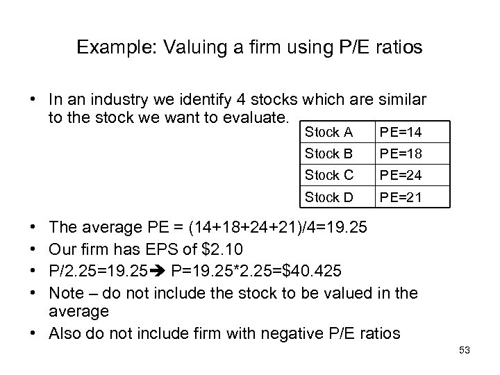Example: Valuing a firm using P/E ratios • In an industry we identify 4 stocks which are similar to the stock we want to evaluate. Stock A PE=14 Stock B PE=18 Stock C PE=24 Stock D PE=21 • • The average PE = (14+18+24+21)/4=19. 25 Our firm has EPS of $2. 10 P/2. 25=19. 25 P=19. 25*2. 25=$40. 425 Note – do not include the stock to be valued in the average • Also do not include firm with negative P/E ratios 53

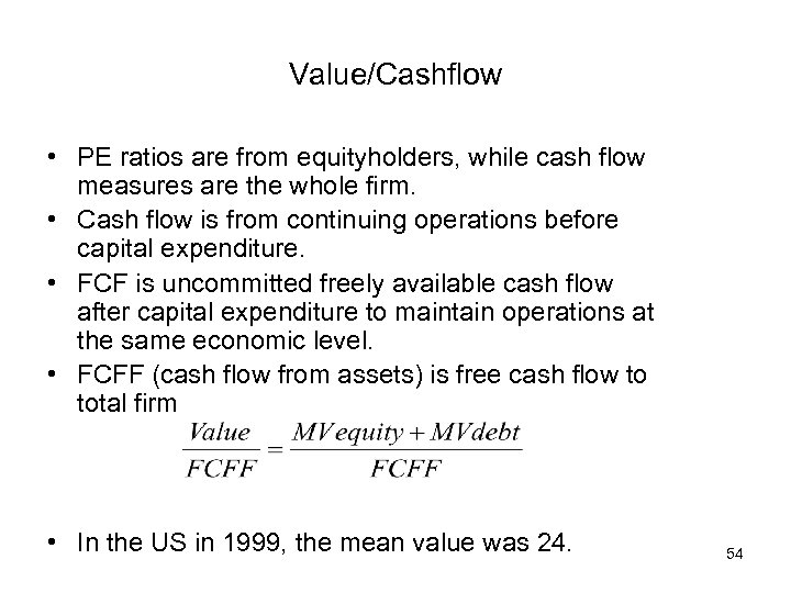Value/Cashflow • PE ratios are from equityholders, while cash flow measures are the whole firm. • Cash flow is from continuing operations before capital expenditure. • FCF is uncommitted freely available cash flow after capital expenditure to maintain operations at the same economic level. • FCFF (cash flow from assets) is free cash flow to total firm • In the US in 1999, the mean value was 24. 54

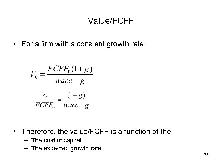Value/FCFF • For a firm with a constant growth rate • Therefore, the value/FCFF is a function of the – The cost of capital – The expected growth rate 55

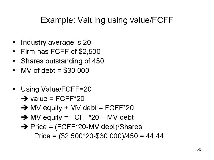Example: Valuing using value/FCFF • • Industry average is 20 Firm has FCFF of $2, 500 Shares outstanding of 450 MV of debt = $30, 000 • Using Value/FCFF=20 value = FCFF*20 MV equity + MV debt = FCFF*20 MV equity = FCFF*20 – MV debt Price = (FCFF*20 -MV debt)/Shares Price = ($2, 500*20 -$30, 000)/450 = 44. 44 56

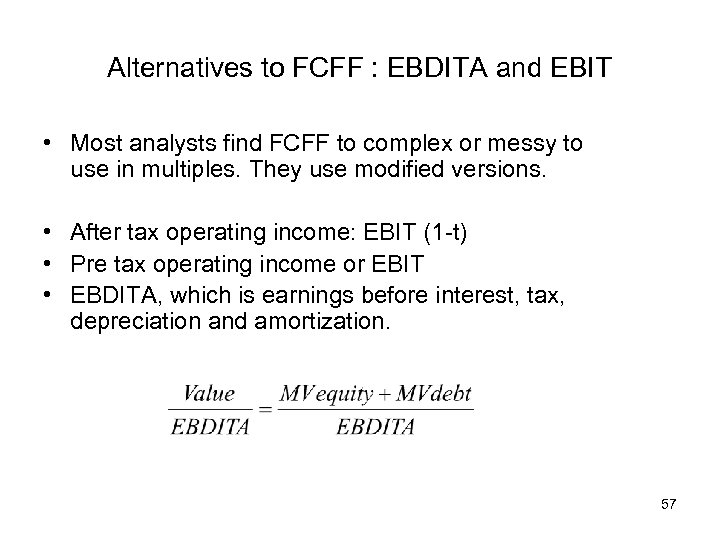Alternatives to FCFF : EBDITA and EBIT • Most analysts find FCFF to complex or messy to use in multiples. They use modified versions. • After tax operating income: EBIT (1 -t) • Pre tax operating income or EBIT • EBDITA, which is earnings before interest, tax, depreciation and amortization. 57

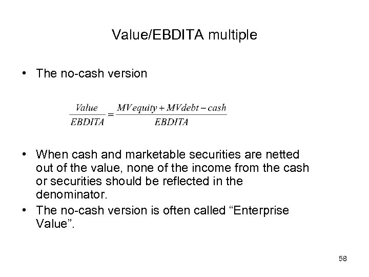Value/EBDITA multiple • The no-cash version • When cash and marketable securities are netted out of the value, none of the income from the cash or securities should be reflected in the denominator. • The no-cash version is often called “Enterprise Value”. 58

Enterprise Value • EV = market value of equity + market value of debt – cash and marketable securities • Many companies who have just conducted an IPOs have huge amount of cash – a “war chest” • EV excludes this cash from value of the firm • Cash +MV of non-cash assets = MV debt + MV equity - Cash For example: Nasdaq AWRE (did IPO in 1996) Its 1996 cash was $31. 1 million, Total assets = $40. 1 million, Debt=0 EV=$9 million. For young firms it is common to use EV instead of Value. 59

Reasons for increased use of Value/EBDITA 1. The multiple can be computed even for firms that are reporting net losses, since EBDITA are usually positive. 2. More appropriate than the PE ratio of high growth firms. 3. Allows for comparison across firms with different financial leverage. 60

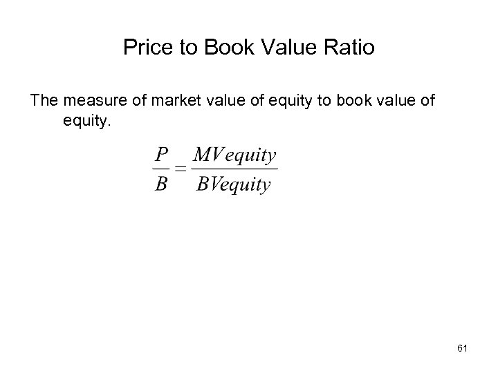Price to Book Value Ratio The measure of market value of equity to book value of equity. 61

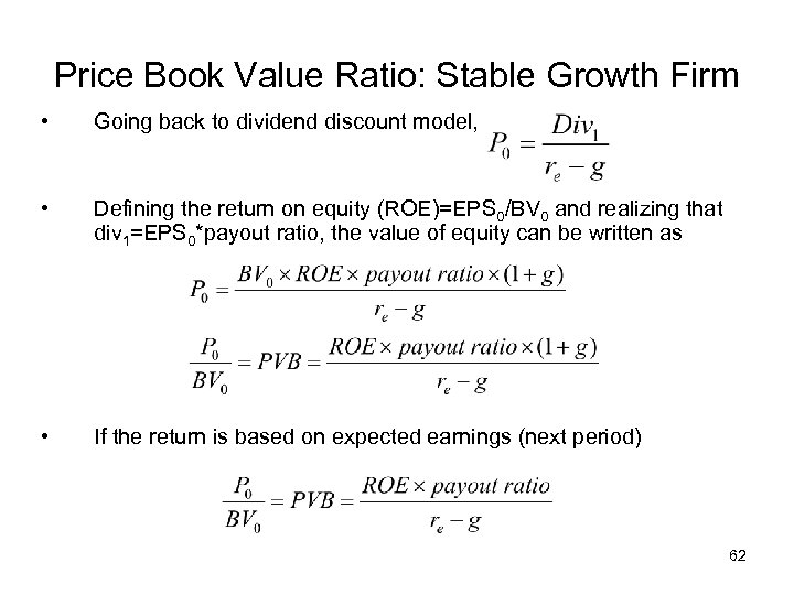Price Book Value Ratio: Stable Growth Firm • Going back to dividend discount model, • Defining the return on equity (ROE)=EPS 0/BV 0 and realizing that div 1=EPS 0*payout ratio, the value of equity can be written as • If the return is based on expected earnings (next period) 62

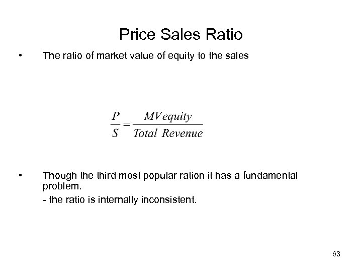Price Sales Ratio • The ratio of market value of equity to the sales • Though the third most popular ration it has a fundamental problem. - the ratio is internally inconsistent. 63

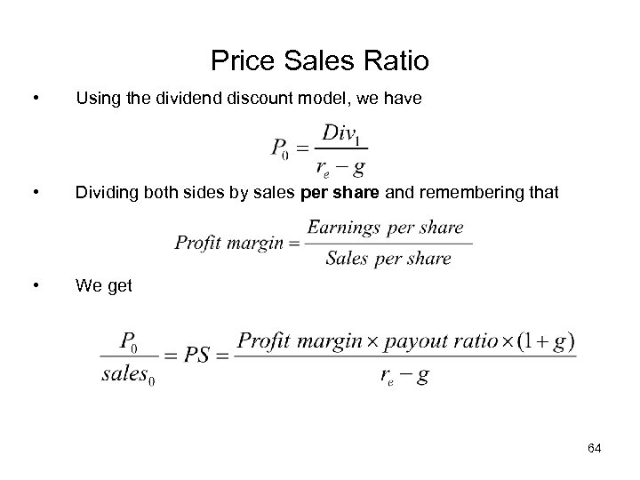Price Sales Ratio • Using the dividend discount model, we have • Dividing both sides by sales per share and remembering that • We get 64

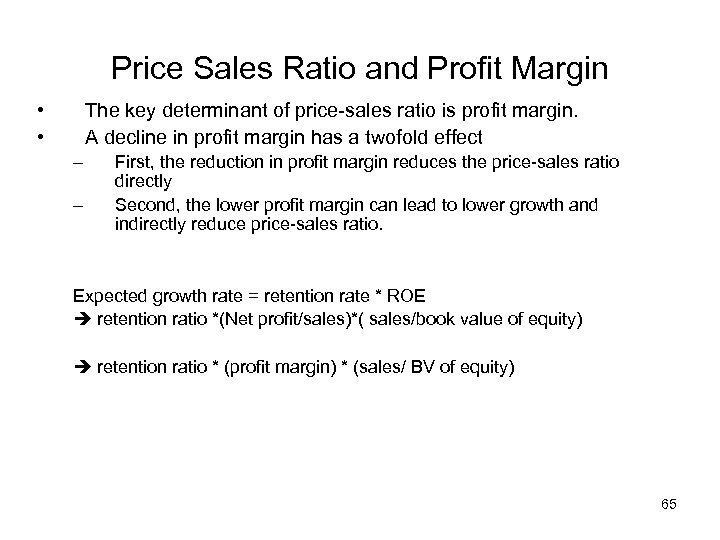Price Sales Ratio and Profit Margin • • The key determinant of price-sales ratio is profit margin. A decline in profit margin has a twofold effect – – First, the reduction in profit margin reduces the price-sales ratio directly Second, the lower profit margin can lead to lower growth and indirectly reduce price-sales ratio. Expected growth rate = retention rate * ROE retention ratio *(Net profit/sales)*( sales/book value of equity) retention ratio * (profit margin) * (sales/ BV of equity) 65

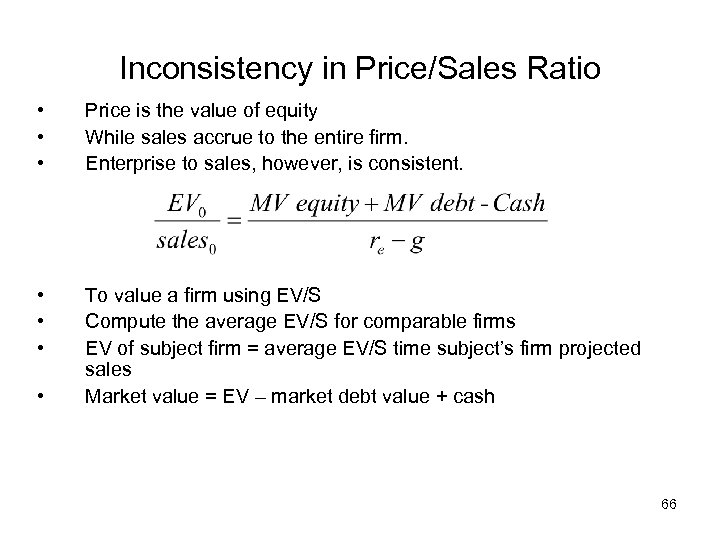Inconsistency in Price/Sales Ratio • • • Price is the value of equity While sales accrue to the entire firm. Enterprise to sales, however, is consistent. • • • To value a firm using EV/S Compute the average EV/S for comparable firms EV of subject firm = average EV/S time subject’s firm projected sales Market value = EV – market debt value + cash • 66

Choosing between the Multiples • • There are dozen of multiples There are three choices – Use a simple average of the valuations obtained using a number of different multiples – Use a weighted average of the valuations obtained using a number of different multiples (one ratio may be more important than another) – Choose one of the multiples and base your valuation based on that multiple (usually the best way as you provide some insights why that multiple is important – remember car industry video segment) 67

Real Options – Chapter 22 4 types of “Real Options” 1 - The opportunity to expand make follow-up investments. 2 - The opportunity to “wait” and invest later. 3 - The opportunity to shrink or abandon a project. 4 - The opportunity to vary the mix of the firm’s output or production methods. Value “Real Option” = NPV with option - NPV w/o option 68

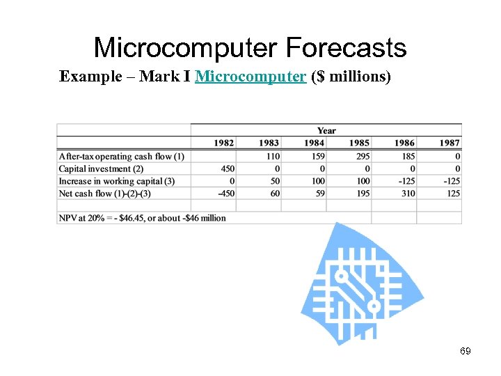Microcomputer Forecasts Example – Mark I Microcomputer ($ millions) 69

Microcomputer Forecasts Your comment – If we do not launch the Mark I, it will probably be too expensive to enter the micro market later, when Apple and IBM are firmly established. In other words, we lose the option to produce the Mark II Microcomputer. Assumptions: 1) The decision on Mark II will take place 3 years from now, in 1985. 2) The investment in Mark II is double that of Mark I, i. e. , $900 m. 3) Forecasted cash flows are also doubled, with PV of $807 m in 1985, and $467 m in 1982. 4) Assume standard deviation of 35% for cashflow uncertainty. 5) Annual riskfree rate is 10%. 70

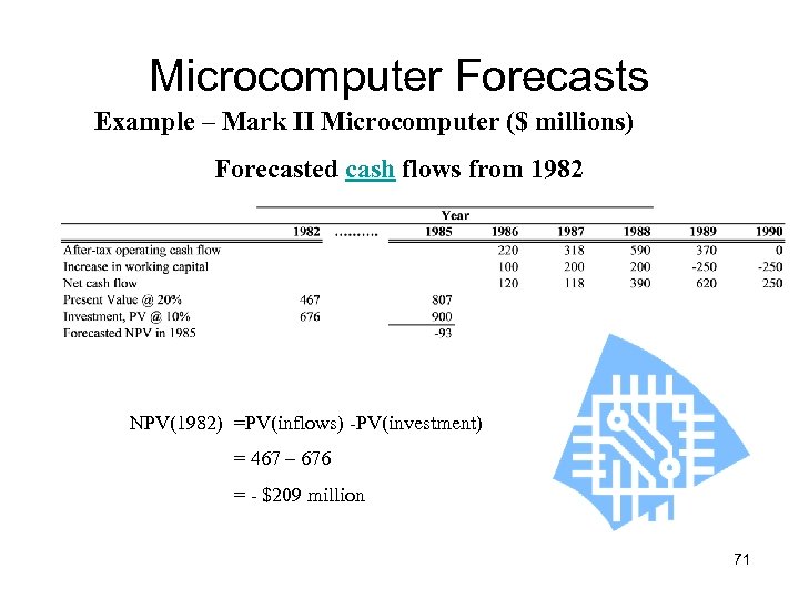Microcomputer Forecasts Example – Mark II Microcomputer ($ millions) Forecasted cash flows from 1982 NPV(1982) =PV(inflows) -PV(investment) = 467 – 676 = - $209 million 71

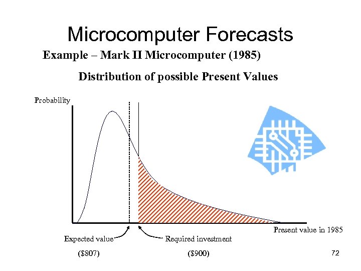Microcomputer Forecasts Example – Mark II Microcomputer (1985) Distribution of possible Present Values Probability Present value in 1985 Expected value Required investment ($807) ($900) 72

Restaurant Investment You have negotiated a deal with a major restaurant chain to open one of its restaurants in your home town. The terms of the contract specify that you must open the restaurant either immediately or in exactly one year. If you do neither, you lose the right to open the restaurant. It will cost you $5 million to open the restaurant, whether you open it now or in one year. If you open the restaurant immediately, you expect to generate $600, 000 in free cash flow the first year. While future cash flow vary with the consumer tastes, they are expected to grow at a rate of 2% per year. The risk free rate is 5% , the appropriate cost of capital for this investment is 12%, and the return volatility of publicly traded comparable firms is 40%. a. What is the NPV of the project if you open today? b. What is the NPV of the project if you delay the opening and wait the year? 73

Option Valuation There are two ways to calculate the value of an option. 1. Find the combination of stock and loan that replicates an investment in the option. Since the two strategies give identical payoffs in the future, they must sell for the same price today. This is basically how one derives the B&S formula. 2. Since option pricing does not depend on risk aversion of investors, we can pretend that all investors are indifferent to risk, work out the expected future value of the option in such a world, and discount it back at the risk-free rate to give the current value. This is called risk-neutral pricing. 74

Growth Option Start. Up Incorporated is a new company whose only asset is a patent on a new drug. If produced, the drug will generate certain profits of $1 million per year for the life of the patent, which is 17 years (after then, competition will drive profits to zero). It will cost $10 million to produce the drug. Assume that the yield on a 17 year risk free annuity is currently 8% per year. a. What is the value of the patent? b. Now assume interest rates will change in exactly one year. At that time, all risk-free interest rates in the economy will be either 10% per year or 5% per year, and then will remain at that level forever. What is the value of the patent? 75

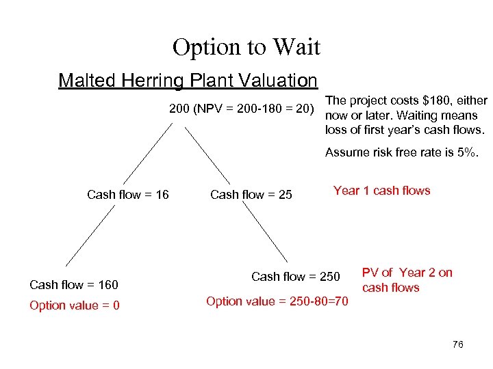Option to Wait Malted Herring Plant Valuation 200 (NPV = 200 -180 = 20) The project costs $180, either now or later. Waiting means loss of first year’s cash flows. Assume risk free rate is 5%. Cash flow = 160 Option value = 0 Cash flow = 25 Year 1 cash flows Cash flow = 250 PV of Year 2 on cash flows Option value = 250 -80=70 76

Option to Wait Real Estate Development Suppose you own a slot of vacant land that can be used for a hotel or an office building, but not for both. To convert a hotel to an office, or an office to a hotel involves high costs. You may be reluctant to invest, even if both investments have positive NPVs. 77

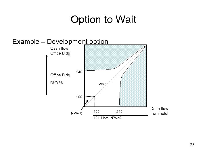Option to Wait Example – Development option Cash flow Office Bldg 240 NPV>0 Wait 100 NPV<0 100 240 Cash flow from hotel 101 Hotel NPV>0 78

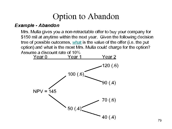Option to Abandon Example - Abandon Mrs. Mulla gives you a non-retractable offer to buy your company for $150 mil at anytime within the next year. Given the following decision tree of possible outcomes, what is the value of the offer (i. e. the put option) and what is the most Mrs. Mulla could charge for the option? Assume a discount rate of 10% Year 0 Year 1 Year 2 120 (. 6) 100 (. 6) 90 (. 4) NPV = 145 70 (. 6) 50 (. 4) 40 (. 4) 79

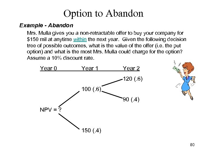Option to Abandon Example - Abandon Mrs. Mulla gives you a non-retractable offer to buy your company for $150 mil at anytime within the next year. Given the following decision tree of possible outcomes, what is the value of the offer (i. e. the put option) and what is the most Mrs. Mulla could charge for the option? Assume a 10% discount rate. Year 0 Year 1 Year 2 120 (. 6) 100 (. 6) 90 (. 4) NPV = ? 150 (. 4) 80

The Zircon Subductor Project Information: 1) The investment required is $12 m and may last up to 10 years. Throughout the project life the company can sell the asset for a certain salvage value that depreciates over time. At year 10 it is worth $5. 99 m. 2) Revenues: $2. 5 million per year (at today’s prices). Revenues are proportional to price. Risk-adjusted rate is 9%. 3) The fixed cost are constant at $700 k per year and are risk fee. Risk free discount rate is 6%. 4) NPV without abandonment option is negative at $ -1. 108 m. 5) Prices of Subductor follow a random walk with a 20% standard deviation. Assuming log normal distribution this leads to a binomial tree of either 22% up or 82% down. 81

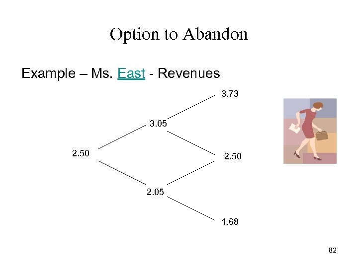Option to Abandon Example – Ms. East - Revenues 3. 73 3. 05 2. 50 2. 05 1. 68 82

Option to Abandon Solving Procedure: 1) Have the salvage value in each of the years 1 -10 (e. g. , 5% deprecation per year) 2) Start at far right (year t=10) and work recursively backwards to the present. At year 10, the project is valued at the ending salvage value. 3) Work backwards to year t-1, use risk neutral probabilities to calculate PV of continuation project. 4) If salvage value of year t-1> PV of continuation value, than the value at the nod=salvage value. If salvage value< PV of continuation project then value at nod = PV of continuation project. 83

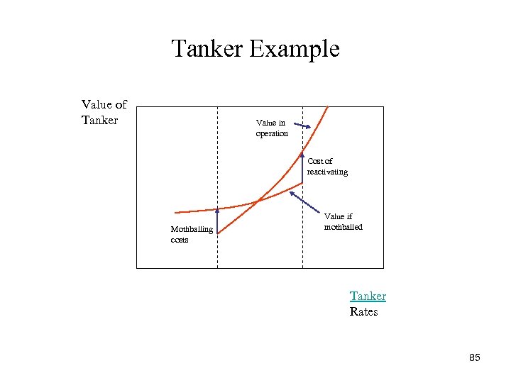
Temporary Abandonment • Suppose you own an oil tanker and you charter your service. The tanker costs $5 million a year to operate and produces $5. 25 in revenue. • What happens if tanker rates go down by 10%, do you close the business immediately? 84

Tanker Example Value of Tanker Value in operation Cost of reactivating Mothballing costs Value if mothballed Tanker Rates 85