34cd592f8741fa96ee16aa782a4b41b1.ppt
- Количество слайдов: 56
 Chapter 18 Simple Linear Regression and Correlation Copyright © 2009 Cengage Learning 16. 1
 Regression Analysis… Our problem objective is to analyze the relationship between interval variables; regression analysis is the first tool we will study. Regression analysis is used to predict the value of one variable (the dependent variable) on the basis of other variables (the independent variables). Dependent variable: denoted Y Independent variables: denoted X 1, X 2, …, Xk Copyright © 2009 Cengage Learning 16. 2
 Correlation Analysis… If we are interested only in determining whether a relationship exists, we employ correlation analysis, a technique introduced earlier. This chapter will examine the relationship between two variables, sometimes called simple linear regression. Mathematical equations describing these relationships are also called models, and they fall into two types: deterministic or probabilistic. Copyright © 2009 Cengage Learning 16. 3
 Model Types… Deterministic Model: an equation or set of equations that allow us to fully determine the value of the dependent variable from the values of the independent variables. Contrast this with… Probabilistic Model: a method used to capture the randomness that is part of a real-life process. E. g. do all houses of the same size (measured in square feet) sell for exactly the same price? Copyright © 2009 Cengage Learning 16. 4
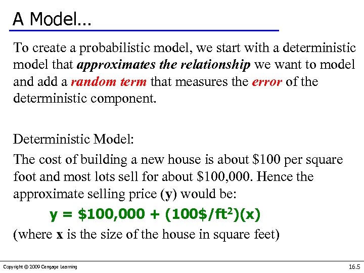 A Model… To create a probabilistic model, we start with a deterministic model that approximates the relationship we want to model and add a random term that measures the error of the deterministic component. Deterministic Model: The cost of building a new house is about $100 per square foot and most lots sell for about $100, 000. Hence the approximate selling price (y) would be: y = $100, 000 + (100$/ft 2)(x) (where x is the size of the house in square feet) Copyright © 2009 Cengage Learning 16. 5
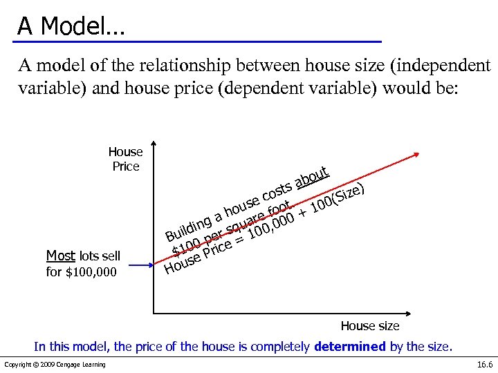 A Model… A model of the relationship between house size (independent variable) and house price (dependent variable) would be: House Price Most lots sell for $100, 000 out ab s ost ize) c (S use foot. 100 o a h are 00 + g 0 ildin er squ 100, u B 0 p 0 Price = $1 e s House size In this model, the price of the house is completely determined by the size. Copyright © 2009 Cengage Learning 16. 6
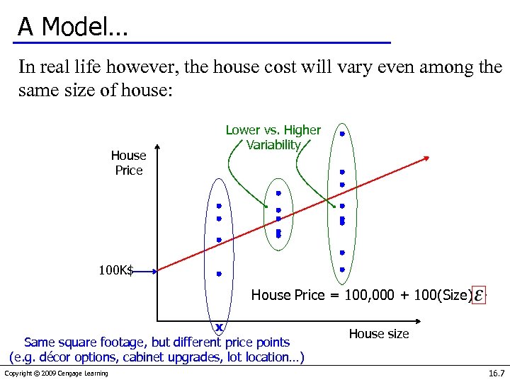 A Model… In real life however, the house cost will vary even among the same size of house: House Price Lower vs. Higher Variability 100 K$ House Price = 100, 000 + 100(Size) + x Same square footage, but different price points (e. g. décor options, cabinet upgrades, lot location…) Copyright © 2009 Cengage Learning House size 16. 7
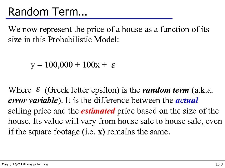 Random Term… We now represent the price of a house as a function of its size in this Probabilistic Model: y = 100, 000 + 100 x + Where (Greek letter epsilon) is the random term (a. k. a. error variable). It is the difference between the actual selling price and the estimated price based on the size of the house. Its value will vary from house sale to house sale, even if the square footage (i. e. x) remains the same. Copyright © 2009 Cengage Learning 16. 8
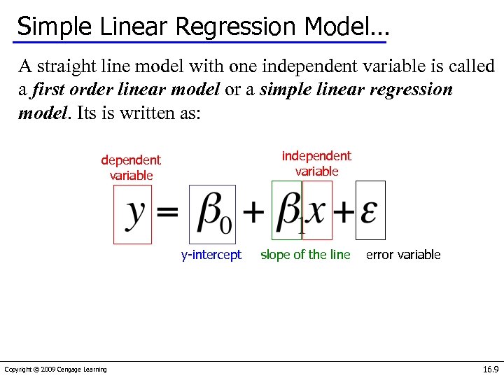 Simple Linear Regression Model… A straight line model with one independent variable is called a first order linear model or a simple linear regression model. Its is written as: independent variable y-intercept Copyright © 2009 Cengage Learning slope of the line error variable 16. 9
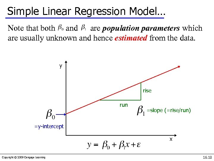 Simple Linear Regression Model… Note that both and are population parameters which are usually unknown and hence estimated from the data. y rise run =slope (=rise/run) =y-intercept x Copyright © 2009 Cengage Learning 16. 10
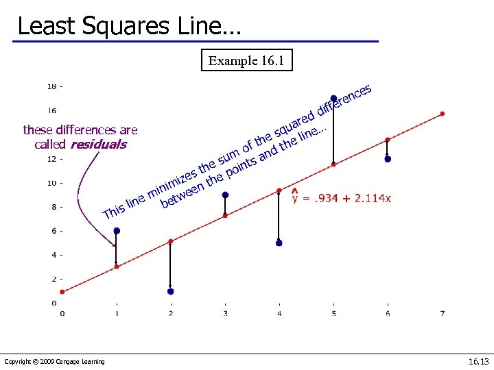
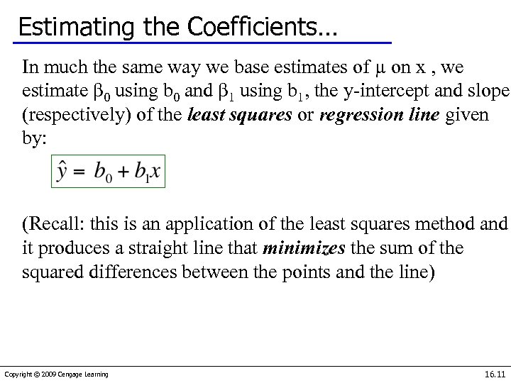 Estimating the Coefficients… In much the same way we base estimates of µ on x , we estimate β 0 using b 0 and β 1 using b 1, the y-intercept and slope (respectively) of the least squares or regression line given by: (Recall: this is an application of the least squares method and it produces a straight line that minimizes the sum of the squared differences between the points and the line) Copyright © 2009 Cengage Learning 16. 11
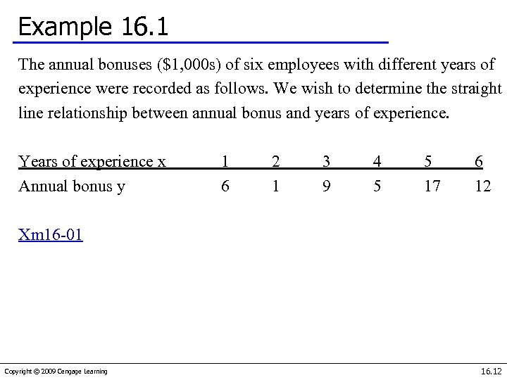 Example 16. 1 The annual bonuses ($1, 000 s) of six employees with different years of experience were recorded as follows. We wish to determine the straight line relationship between annual bonus and years of experience. Years of experience x Annual bonus y 1 6 2 1 3 9 4 5 5 17 6 12 Xm 16 -01 Copyright © 2009 Cengage Learning 16. 12
 Least Squares Line… Example 16. 1 ces en r iffe d ed r these differences are qua ine… s the l called residuals of nd a um e s oints s th e p ze imi en th min twe ne be s li Thi Copyright © 2009 Cengage Learning 16. 13
 Example 16. 2… Car dealers across North America use the "Red Book" to help them determine the value of used cars that their customers trade in when purchasing new cars. The book, which is published monthly, lists the trade-in values for all basic models of cars. It provides alternative values for each car model according to its condition and optional features. The values are determined on the basis of the average paid at recent used-car auctions, the source of supply for many used-car dealers. Copyright © 2009 Cengage Learning 16. 14
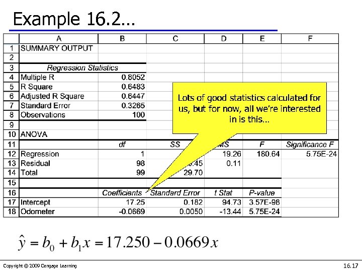
 Example 16. 2… However, the Red Book does not indicate the value determined by the odometer reading, despite the fact that a critical factor for used-car buyers is how far the car has been driven. To examine this issue, a used-car dealer randomly selected 100 threeyear old Toyota Camrys that were sold at auction during the past month. The dealer recorded the price ($1, 000) and the number of miles (thousands) on the odometer. (Xm 16 -02). The dealer wants to find the regression line. Copyright © 2009 Cengage Learning 16. 15
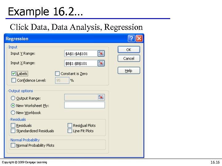 Example 16. 2… Click Data, Data Analysis, Regression Copyright © 2009 Cengage Learning 16. 16
 Example 16. 2… Copyright © 2009 Cengage Learning 16. 17
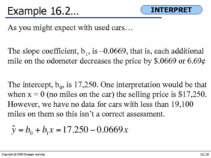 Example 16. 2… INTERPRET As you might expect with used cars… The slope coefficient, b 1, is – 0. 0669, that is, each additional mile on the odometer decreases the price by $. 0669 or 6. 69¢ The intercept, b 0, is 17, 250. One interpretation would be that when x = 0 (no miles on the car) the selling price is $17, 250. However, we have no data for cars with less than 19, 100 miles on them so this isn’t a correct assessment. Copyright © 2009 Cengage Learning 16. 18
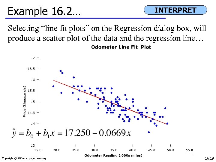 Example 16. 2… INTERPRET Selecting “line fit plots” on the Regression dialog box, will produce a scatter plot of the data and the regression line… Copyright © 2009 Cengage Learning 16. 19
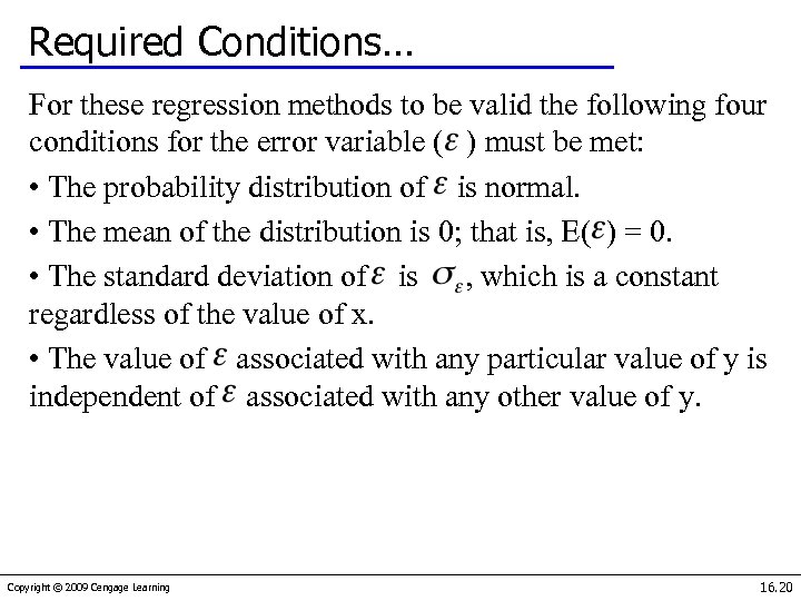 Required Conditions… For these regression methods to be valid the following four conditions for the error variable ( ) must be met: • The probability distribution of is normal. • The mean of the distribution is 0; that is, E( ) = 0. • The standard deviation of is , which is a constant regardless of the value of x. • The value of associated with any particular value of y is independent of associated with any other value of y. Copyright © 2009 Cengage Learning 16. 20
 Assessing the Model… The least squares method will always produce a straight line, even if there is no relationship between the variables, or if the relationship is something other than linear. Hence, in addition to determining the coefficients of the least squares line, we need to assess it to see how well it “fits” the data. We’ll see these evaluation methods now. They’re based on the sum of squares for errors (SSE). Copyright © 2009 Cengage Learning 16. 21
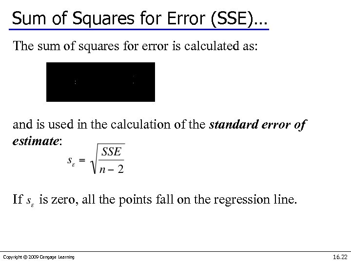 Sum of Squares for Error (SSE)… The sum of squares for error is calculated as: and is used in the calculation of the standard error of estimate: If is zero, all the points fall on the regression line. Copyright © 2009 Cengage Learning 16. 22
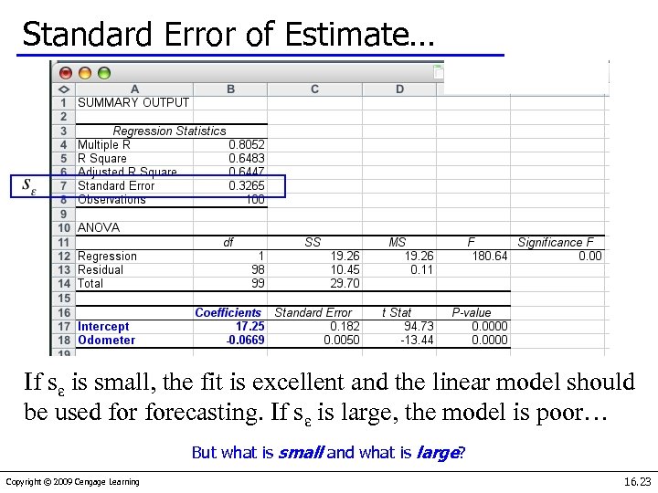 Standard Error of Estimate… If sε is small, the fit is excellent and the linear model should be used forecasting. If sε is large, the model is poor… But what is small and what is large? Copyright © 2009 Cengage Learning 16. 23
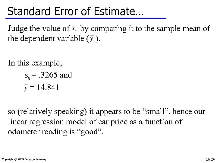 Standard Error of Estimate… Judge the value of by comparing it to the sample mean of the dependent variable ( ). In this example, sε =. 3265 and = 14. 841 so (relatively speaking) it appears to be “small”, hence our linear regression model of car price as a function of odometer reading is “good”. Copyright © 2009 Cengage Learning 16. 24
 Testing the Slope… If no linear relationship exists between the two variables, we would expect the regression line to be horizontal, that is, to have a slope of zero. We want to see if there is a linear relationship, i. e. we want to see if the slope (β 1) is something other than zero. Our research hypothesis becomes: H 1: β 1 ≠ 0 Thus the null hypothesis becomes: H 0: β 1 = 0 Copyright © 2009 Cengage Learning 16. 25
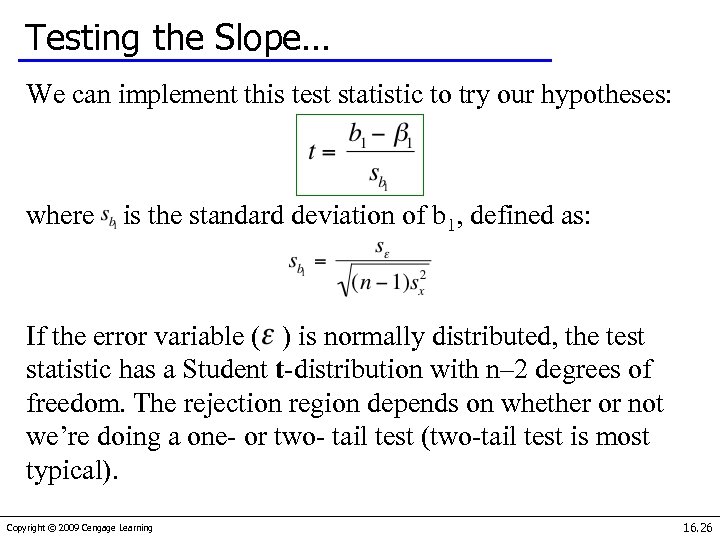 Testing the Slope… We can implement this test statistic to try our hypotheses: where is the standard deviation of b 1, defined as: If the error variable ( ) is normally distributed, the test statistic has a Student t-distribution with n– 2 degrees of freedom. The rejection region depends on whether or not we’re doing a one- or two- tail test (two-tail test is most typical). Copyright © 2009 Cengage Learning 16. 26
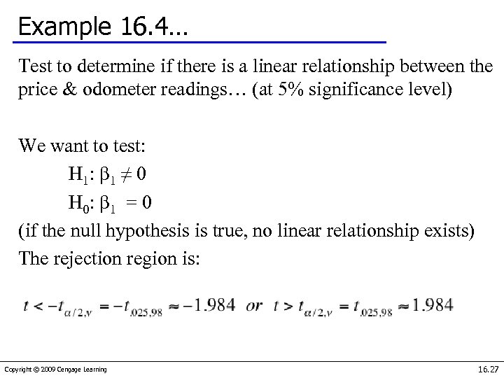 Example 16. 4… Test to determine if there is a linear relationship between the price & odometer readings… (at 5% significance level) We want to test: H 1: β 1 ≠ 0 H 0: β 1 = 0 (if the null hypothesis is true, no linear relationship exists) The rejection region is: Copyright © 2009 Cengage Learning 16. 27
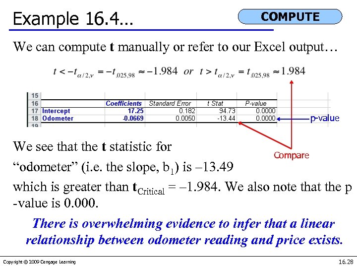 Example 16. 4… COMPUTE We can compute t manually or refer to our Excel output… p-value We see that the t statistic for Compare “odometer” (i. e. the slope, b 1) is – 13. 49 which is greater than t. Critical = – 1. 984. We also note that the p -value is 0. 000. There is overwhelming evidence to infer that a linear relationship between odometer reading and price exists. Copyright © 2009 Cengage Learning 16. 28
 Testing the Slope… If we wish to test for positive or negative linear relationships we conduct one-tail tests, i. e. our research hypothesis become: H 1: β 1 < 0 (testing for a negative slope) or H 1: β 1 >0 (testing for a positive slope) Of course, the null hypothesis remains: H 0: β 1 = 0. Copyright © 2009 Cengage Learning 16. 29
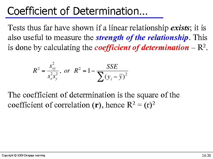 Coefficient of Determination… Tests thus far have shown if a linear relationship exists; it is also useful to measure the strength of the relationship. This is done by calculating the coefficient of determination – R 2. The coefficient of determination is the square of the coefficient of correlation (r), hence R 2 = (r)2 Copyright © 2009 Cengage Learning 16. 30
 Coefficient of Determination… As we did with analysis of variance, we can partition the variation in y into two parts: Variation in y = SSE + SSR SSE – Sum of Squares Error – measures the amount of variation in y that remains unexplained (i. e. due to error) SSR – Sum of Squares Regression – measures the amount of variation in y explained by variation in the independent variable x. Copyright © 2009 Cengage Learning 16. 31
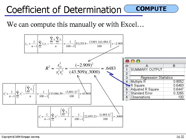 Coefficient of Determination COMPUTE We can compute this manually or with Excel… Copyright © 2009 Cengage Learning 16. 32
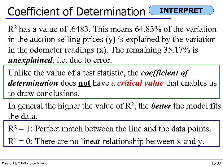 Coefficient of Determination INTERPRET R 2 has a value of. 6483. This means 64. 83% of the variation in the auction selling prices (y) is explained by the variation in the odometer readings (x). The remaining 35. 17% is unexplained, i. e. due to error. Unlike the value of a test statistic, the coefficient of determination does not have a critical value that enables us to draw conclusions. In general the higher the value of R 2, the better the model fits the data. R 2 = 1: Perfect match between the line and the data points. R 2 = 0: There are no linear relationship between x and y. Copyright © 2009 Cengage Learning 16. 33
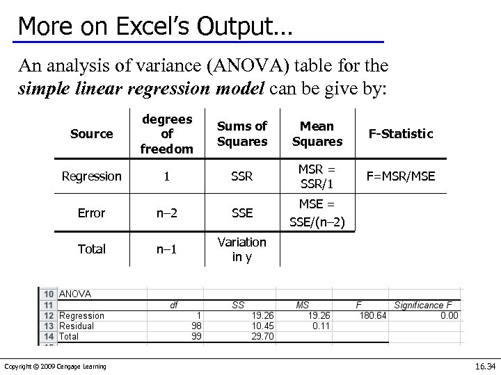 More on Excel’s Output… An analysis of variance (ANOVA) table for the simple linear regression model can be give by: Source degrees of freedom Sums of Squares Mean Squares F-Statistic Regression 1 SSR MSR = SSR/1 F=MSR/MSE = SSE/(n– 2) Error n– 2 SSE Total n– 1 Variation in y Copyright © 2009 Cengage Learning 16. 34
 Coefficient of Correlation We can use the coefficient of correlation (introduced earlier) to test for a linear relationship between two variables. Recall: The coefficient of correlation’s range is between – 1 and +1. • If r = – 1 (negative association) or r = +1 (positive association) every point falls on the regression line. • If r = 0 there is no linear pattern Copyright © 2009 Cengage Learning 16. 35
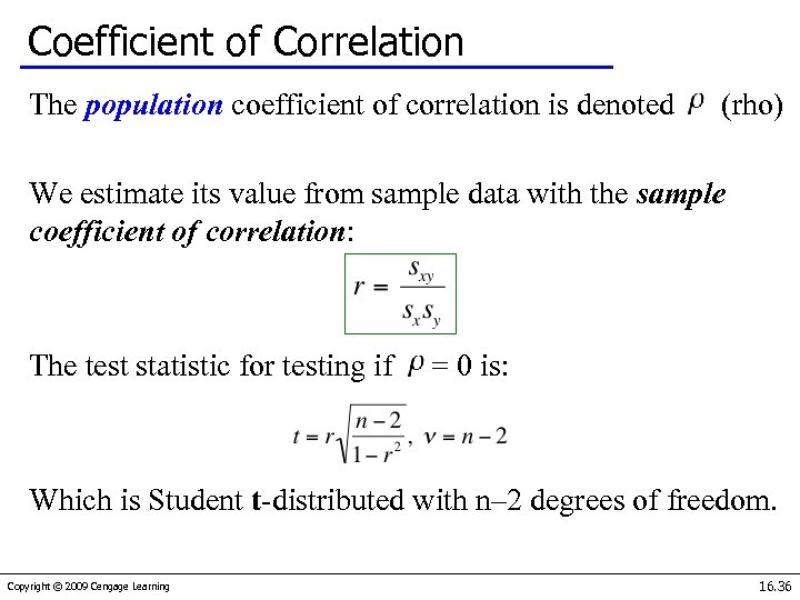 Coefficient of Correlation The population coefficient of correlation is denoted (rho) We estimate its value from sample data with the sample coefficient of correlation: The test statistic for testing if = 0 is: Which is Student t-distributed with n– 2 degrees of freedom. Copyright © 2009 Cengage Learning 16. 36
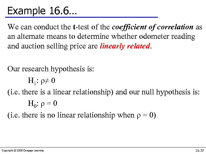 Example 16. 6… We can conduct the t-test of the coefficient of correlation as an alternate means to determine whether odometer reading and auction selling price are linearly related. Our research hypothesis is: H 1: ρ≠ 0 (i. e. there is a linear relationship) and our null hypothesis is: H 0: ρ = 0 (i. e. there is no linear relationship when ρ = 0) Copyright © 2009 Cengage Learning 16. 37
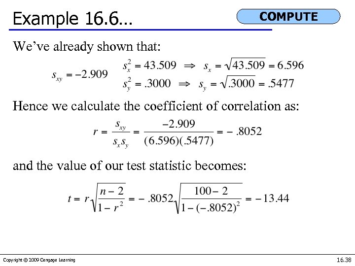 Example 16. 6… COMPUTE We’ve already shown that: Hence we calculate the coefficient of correlation as: and the value of our test statistic becomes: Copyright © 2009 Cengage Learning 16. 38
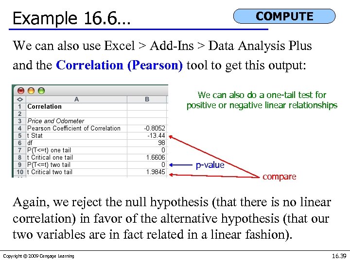 Example 16. 6… COMPUTE We can also use Excel > Add-Ins > Data Analysis Plus and the Correlation (Pearson) tool to get this output: We can also do a one-tail test for positive or negative linear relationships p-value compare Again, we reject the null hypothesis (that there is no linear correlation) in favor of the alternative hypothesis (that our two variables are in fact related in a linear fashion). Copyright © 2009 Cengage Learning 16. 39
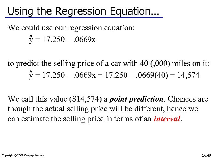 Using the Regression Equation… We could use our regression equation: y = 17. 250 –. 0669 x to predict the selling price of a car with 40 (, 000) miles on it: y = 17. 250 –. 0669 x = 17. 250 –. 0669(40) = 14, 574 We call this value ($14, 574) a point prediction. Chances are though the actual selling price will be different, hence we can estimate the selling price in terms of an interval. Copyright © 2009 Cengage Learning 16. 40
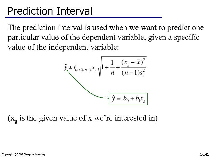 Prediction Interval The prediction interval is used when we want to predict one particular value of the dependent variable, given a specific value of the independent variable: (xg is the given value of x we’re interested in) Copyright © 2009 Cengage Learning 16. 41
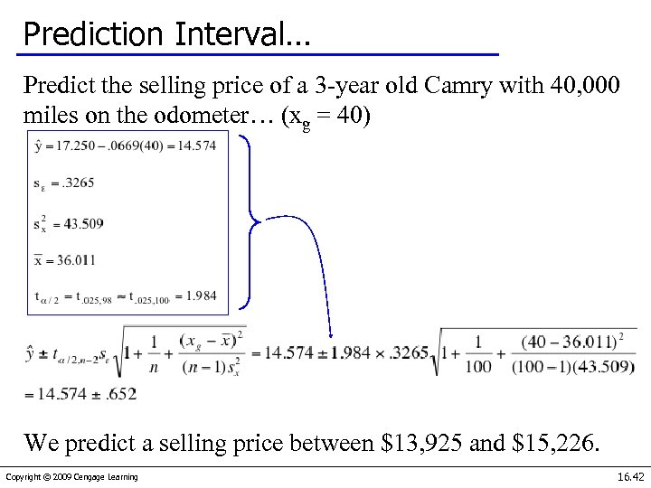 Prediction Interval… Predict the selling price of a 3 -year old Camry with 40, 000 miles on the odometer… (xg = 40) We predict a selling price between $13, 925 and $15, 226. Copyright © 2009 Cengage Learning 16. 42
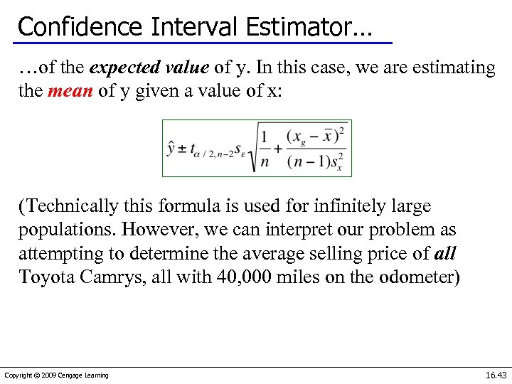 Confidence Interval Estimator… …of the expected value of y. In this case, we are estimating the mean of y given a value of x: (Technically this formula is used for infinitely large populations. However, we can interpret our problem as attempting to determine the average selling price of all Toyota Camrys, all with 40, 000 miles on the odometer) Copyright © 2009 Cengage Learning 16. 43
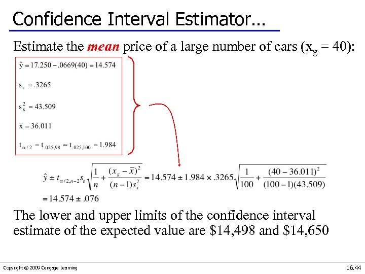 Confidence Interval Estimator… Estimate the mean price of a large number of cars (xg = 40): The lower and upper limits of the confidence interval estimate of the expected value are $14, 498 and $14, 650 Copyright © 2009 Cengage Learning 16. 44
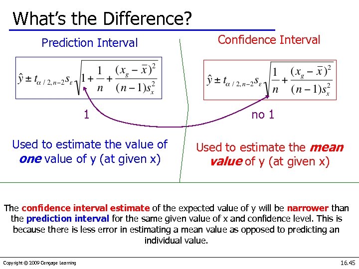 What’s the Difference? Prediction Interval 1 Used to estimate the value of one value of y (at given x) Confidence Interval no 1 Used to estimate the mean value of y (at given x) The confidence interval estimate of the expected value of y will be narrower than the prediction interval for the same given value of x and confidence level. This is because there is less error in estimating a mean value as opposed to predicting an individual value. Copyright © 2009 Cengage Learning 16. 45
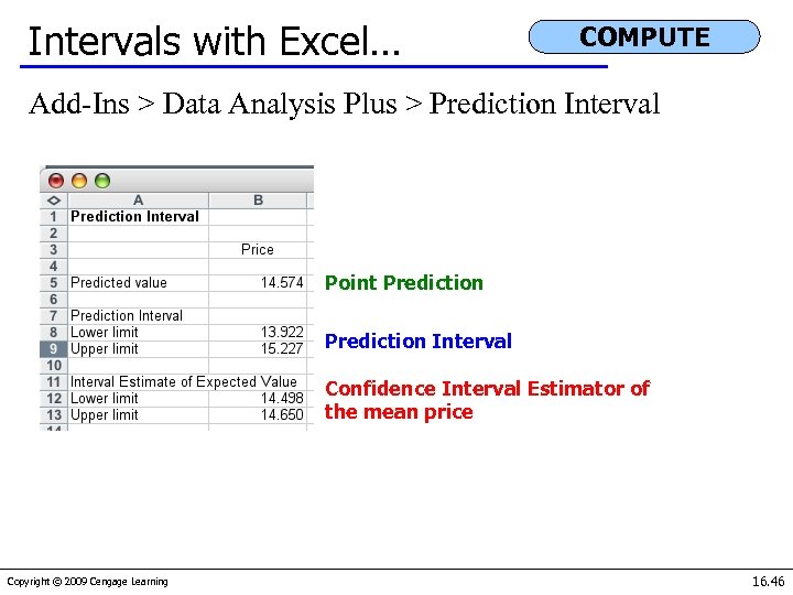 Intervals with Excel… COMPUTE Add-Ins > Data Analysis Plus > Prediction Interval Point Prediction Interval Confidence Interval Estimator of the mean price Copyright © 2009 Cengage Learning 16. 46
 Regression Diagnostics… There are three conditions that are required in order to perform a regression analysis. These are: • The error variable must be normally distributed, • The error variable must have a constant variance, & • The errors must be independent of each other. How can we diagnose violations of these conditions? Residual Analysis, that is, examine the differences between the actual data points and those predicted by the linear equation… Copyright © 2009 Cengage Learning 16. 47
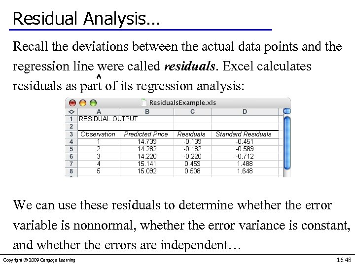 Residual Analysis… Recall the deviations between the actual data points and the regression line were called residuals. Excel calculates residuals as part of its regression analysis: We can use these residuals to determine whether the error variable is nonnormal, whether the error variance is constant, and whether the errors are independent… Copyright © 2009 Cengage Learning 16. 48
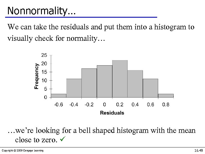 Nonnormality… We can take the residuals and put them into a histogram to visually check for normality… …we’re looking for a bell shaped histogram with the mean close to zero. Copyright © 2009 Cengage Learning 16. 49
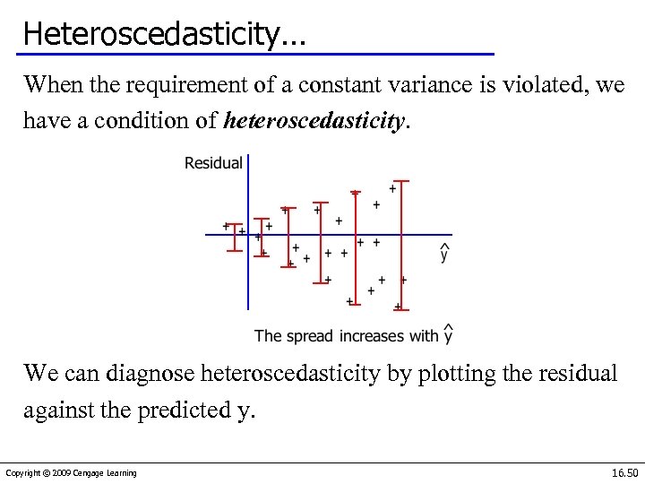 Heteroscedasticity… When the requirement of a constant variance is violated, we have a condition of heteroscedasticity. We can diagnose heteroscedasticity by plotting the residual against the predicted y. Copyright © 2009 Cengage Learning 16. 50
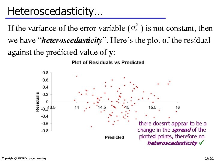 Heteroscedasticity… If the variance of the error variable ( ) is not constant, then we have “heteroscedasticity”. Here’s the plot of the residual against the predicted value of y: there doesn’t appear to be a change in the spread of the plotted points, therefore no heteroscedasticity Copyright © 2009 Cengage Learning 16. 51
 Nonindependence of the Error Variable If we were to observe the auction price of cars every week for, say, a year, that would constitute a time series. When the data are time series, the errors often are correlated. Error terms that are correlated over time are said to be autocorrelated or serially correlated. We can often detect autocorrelation by graphing the residuals against the time periods. If a pattern emerges, it is likely that the independence requirement is violated. Copyright © 2009 Cengage Learning 16. 52
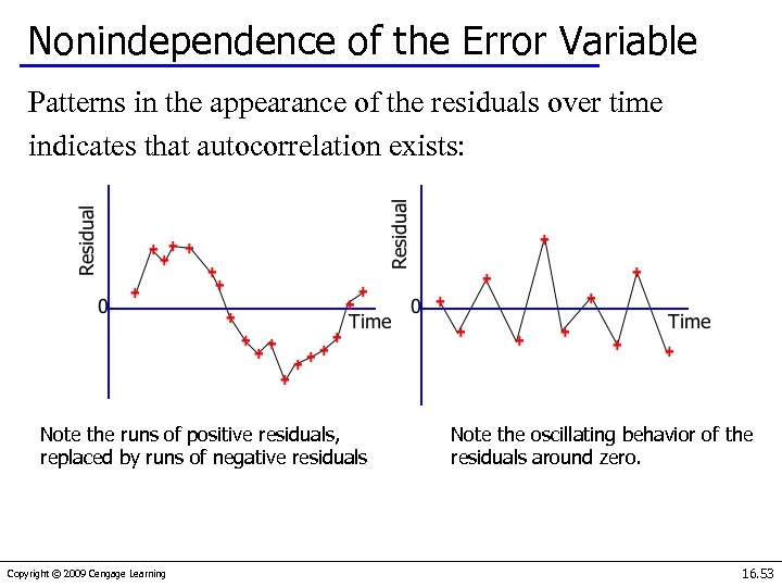 Nonindependence of the Error Variable Patterns in the appearance of the residuals over time indicates that autocorrelation exists: Note the runs of positive residuals, replaced by runs of negative residuals Copyright © 2009 Cengage Learning Note the oscillating behavior of the residuals around zero. 16. 53
 Outliers… An outlier is an observation that is unusually small or unusually large. E. g. our used car example had odometer readings from 19. 1 to 49. 2 thousand miles. Suppose we have a value of only 5, 000 miles (i. e. a car driven by an old person only on Sundays ) — this point is an outlier. Copyright © 2009 Cengage Learning 16. 54
 Outliers… Possible reasons for the existence of outliers include: There was an error in recording the value The point should not have been included in the sample Perhaps the observation is indeed valid. Outliers can be easily identified from a scatter plot. If the absolute value of the standard residual is > 2, we suspect the point may be an outlier and investigate further. They need to be dealt with since they can easily influence the least squares line… Copyright © 2009 Cengage Learning 16. 55
 Procedure for Regression Diagnostics… 1. Develop a model that has a theoretical basis. 2. Gather data for the two variables in the model. 3. Draw the scatter diagram to determine whether a linear model appears to be appropriate. Identify possible outliers. 4. Determine the regression equation. 5. Calculate the residuals and check the required conditions 6. Assess the model’s fit. 7. If the model fits the data, use the regression equation to predict a particular value of the dependent variable and/or estimate its mean. Copyright © 2009 Cengage Learning 16. 56


