b85155f296e26efb7f864d2fc7449b75.ppt
- Количество слайдов: 53
Chapter 18: Data Analysis and Mining Database System Concepts ©Silberschatz, Korth and Sudarshan See www. db-book. com for conditions on re-use
Chapter 18: Data Analysis and Mining n Decision Support Systems n Data Analysis and OLAP n Data Warehousing n Data Mining Database System Concepts - 5 th Edition, Aug 26, 2005 18. 2 ©Silberschatz, Korth and Sudarshan
Database Applications n Transaction processing systems l Record information about transactions 4 Account deposits and withdrawals 4 Sales 4 Course l registations Widely used n Decision support systems l Extract high level summary information from large collections of data l Our topic this week Database System Concepts - 5 th Edition, Aug 26, 2005 18. 3 ©Silberschatz, Korth and Sudarshan
Decision Support Systems n Decision-support systems are used to make business decisions, often based on data collected by on-line transaction-processing systems. n Examples of business decisions: l What items to stock? l What insurance premium to change? l To whom to send advertisements? n Examples of data used for making decisions l Retail sales transaction details l Customer profiles (income, age, gender, etc. ) Database System Concepts - 5 th Edition, Aug 26, 2005 18. 4 ©Silberschatz, Korth and Sudarshan
Decision-Support Systems: Overview n Data analysis tasks are simplified by specialized tools and SQL extensions l Example tasks 4 For each product category and each region, what were the total sales in the last quarter and how do they compare with the same quarter last year 4 As above, for each product category and each customer category n Statistical analysis packages (e. g. , : SAS, S++) can be interfaced with databases l Statistical analysis is a large field, but not covered here n Data mining seeks to discover knowledge automatically in the form of statistical rules and patterns from large databases. n A data warehouse archives information gathered from multiple sources, and stores it under a unified schema, at a single site. l Important for large businesses that generate data from multiple divisions, possibly at multiple sites l Data may also be purchased externally Database System Concepts - 5 th Edition, Aug 26, 2005 18. 5 ©Silberschatz, Korth and Sudarshan
Data Analysis and OLAP n Online Analytical Processing (OLAP) l Interactive analysis of data, allowing data to be summarized and viewed in different ways in an online fashion (with negligible delay) n Data that can be modeled as dimension attributes and measure attributes are called multidimensional data. l Measure attributes 4 measure some value 4 can 4 e. g. l be aggregated upon the attribute number of the sales relation Dimension attributes 4 define the dimensions on which measure attributes (or aggregates thereof) are viewed 4 e. g. the attributes item_name, color, and size of the sales relation Database System Concepts - 5 th Edition, Aug 26, 2005 18. 6 ©Silberschatz, Korth and Sudarshan
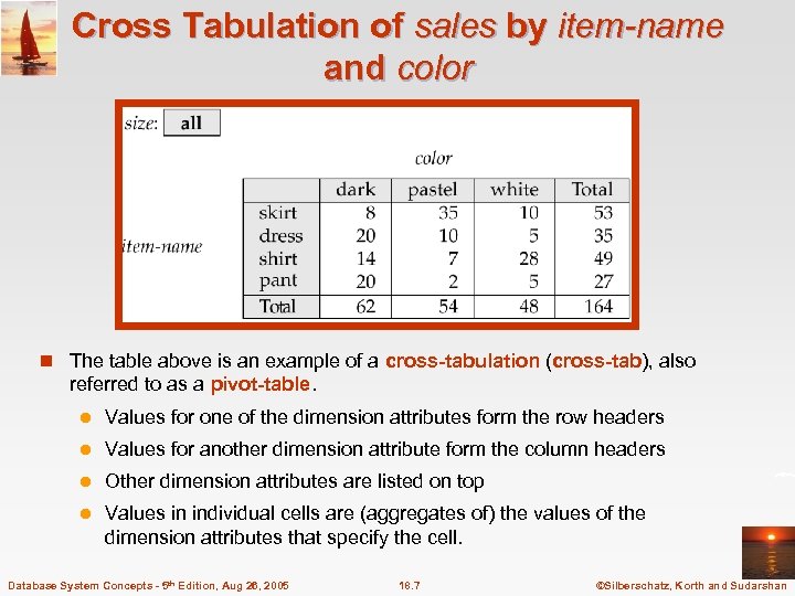
Cross Tabulation of sales by item-name and color n The table above is an example of a cross-tabulation (cross-tab), also referred to as a pivot-table. l Values for one of the dimension attributes form the row headers l Values for another dimension attribute form the column headers l Other dimension attributes are listed on top l Values in individual cells are (aggregates of) the values of the dimension attributes that specify the cell. Database System Concepts - 5 th Edition, Aug 26, 2005 18. 7 ©Silberschatz, Korth and Sudarshan
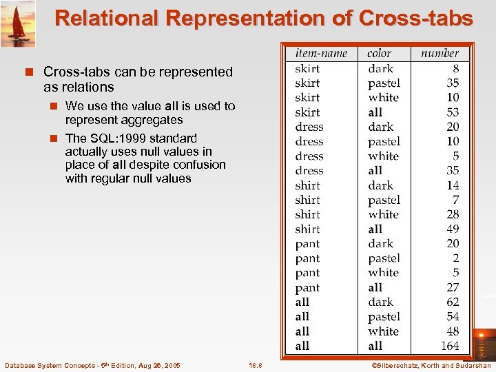
Relational Representation of Cross-tabs n Cross-tabs can be represented as relations n We use the value all is used to represent aggregates n The SQL: 1999 standard actually uses null values in place of all despite confusion with regular null values Database System Concepts - 5 th Edition, Aug 26, 2005 18. 8 ©Silberschatz, Korth and Sudarshan
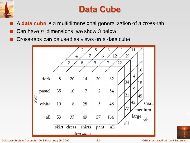
Data Cube n A data cube is a multidimensional generalization of a cross-tab n Can have n dimensions; we show 3 below n Cross-tabs can be used as views on a data cube Database System Concepts - 5 th Edition, Aug 26, 2005 18. 9 ©Silberschatz, Korth and Sudarshan
Online Analytical Processing n Pivoting: changing the dimensions used in a cross-tab is called n Slicing: creating a cross-tab for fixed values only l Sometimes called dicing, particularly when values for multiple dimensions are fixed. n Rollup: moving from finer-granularity data to a coarser granularity n Drill down: The opposite operation - that of moving from coarser- granularity data to finer-granularity data Database System Concepts - 5 th Edition, Aug 26, 2005 18. 10 ©Silberschatz, Korth and Sudarshan
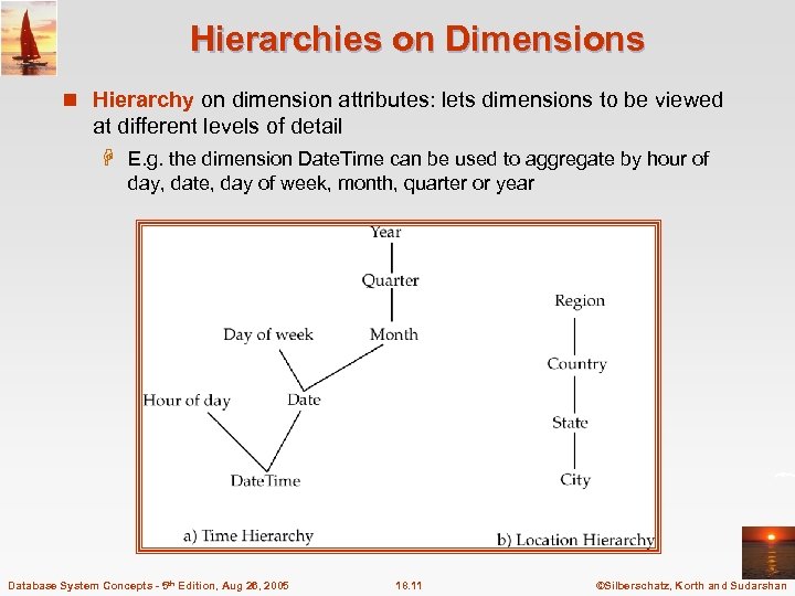
Hierarchies on Dimensions n Hierarchy on dimension attributes: lets dimensions to be viewed at different levels of detail H E. g. the dimension Date. Time can be used to aggregate by hour of day, date, day of week, month, quarter or year Database System Concepts - 5 th Edition, Aug 26, 2005 18. 11 ©Silberschatz, Korth and Sudarshan
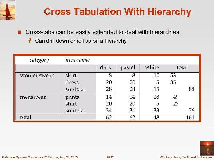
Cross Tabulation With Hierarchy n Cross-tabs can be easily extended to deal with hierarchies H Can drill down or roll up on a hierarchy Database System Concepts - 5 th Edition, Aug 26, 2005 18. 12 ©Silberschatz, Korth and Sudarshan
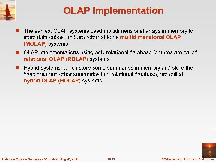
OLAP Implementation n The earliest OLAP systems used multidimensional arrays in memory to store data cubes, and are referred to as multidimensional OLAP (MOLAP) systems. n OLAP implementations using only relational database features are called relational OLAP (ROLAP) systems n Hybrid systems, which store some summaries in memory and store the base data and other summaries in a relational database, are called hybrid OLAP (HOLAP) systems. Database System Concepts - 5 th Edition, Aug 26, 2005 18. 13 ©Silberschatz, Korth and Sudarshan
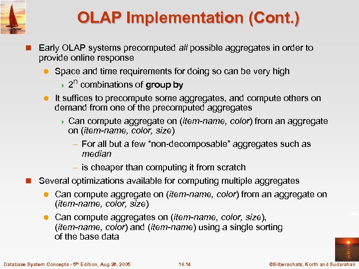
OLAP Implementation (Cont. ) n Early OLAP systems precomputed all possible aggregates in order to provide online response l Space and time requirements for doing so can be very high n 4 2 combinations of group by l It suffices to precompute some aggregates, and compute others on demand from one of the precomputed aggregates 4 Can compute aggregate on (item-name, color) from an aggregate on (item-name, color, size) – For all but a few “non-decomposable” aggregates such as median – is cheaper than computing it from scratch n Several optimizations available for computing multiple aggregates Can compute aggregate on (item-name, color) from an aggregate on (item-name, color, size) l Can compute aggregates on (item-name, color, size), (item-name, color) and (item-name) using a single sorting of the base data l Database System Concepts - 5 th Edition, Aug 26, 2005 18. 14 ©Silberschatz, Korth and Sudarshan
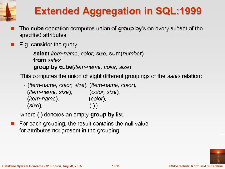
Extended Aggregation in SQL: 1999 n The cube operation computes union of group by’s on every subset of the specified attributes n E. g. consider the query select item-name, color, size, sum(number) from sales group by cube(item-name, color, size) This computes the union of eight different groupings of the sales relation: { (item-name, color, size), (item-name, color), (item-name, size), (color, size), (item-name), (color), (size), ()} where ( ) denotes an empty group by list. n For each grouping, the result contains the null value for attributes not present in the grouping. Database System Concepts - 5 th Edition, Aug 26, 2005 18. 15 ©Silberschatz, Korth and Sudarshan
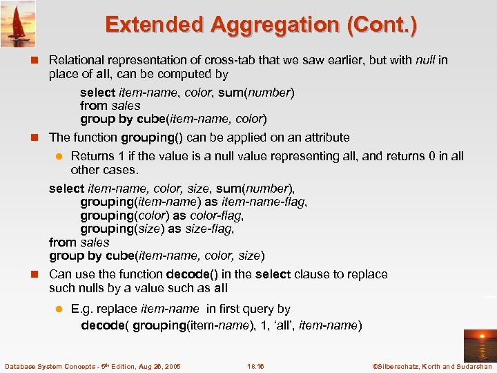
Extended Aggregation (Cont. ) n Relational representation of cross-tab that we saw earlier, but with null in place of all, can be computed by select item-name, color, sum(number) from sales group by cube(item-name, color) n The function grouping() can be applied on an attribute l Returns 1 if the value is a null value representing all, and returns 0 in all other cases. select item-name, color, size, sum(number), grouping(item-name) as item-name-flag, grouping(color) as color-flag, grouping(size) as size-flag, from sales group by cube(item-name, color, size) n Can use the function decode() in the select clause to replace such nulls by a value such as all l E. g. replace item-name in first query by decode( grouping(item-name), 1, ‘all’, item-name) Database System Concepts - 5 th Edition, Aug 26, 2005 18. 16 ©Silberschatz, Korth and Sudarshan
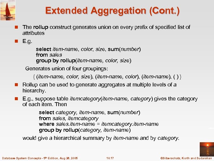
Extended Aggregation (Cont. ) n The rollup construct generates union on every prefix of specified list of attributes n E. g. select item-name, color, size, sum(number) from sales group by rollup(item-name, color, size) Generates union of four groupings: { (item-name, color, size), (item-name, color), (item-name), ( ) } n Rollup can be used to generate aggregates at multiple levels of a hierarchy. n E. g. , suppose table itemcategory(item-name, category) gives the category of each item. Then select category, item-name, sum(number) from sales, itemcategory where sales. item-name = itemcategory. item-name group by rollup(category, item-name) would give a hierarchical summary by item-name and by category. Database System Concepts - 5 th Edition, Aug 26, 2005 18. 17 ©Silberschatz, Korth and Sudarshan
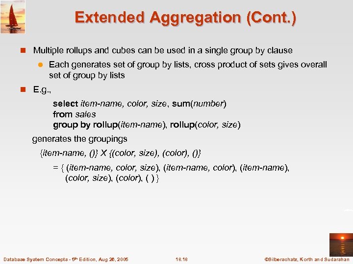
Extended Aggregation (Cont. ) n Multiple rollups and cubes can be used in a single group by clause l Each generates set of group by lists, cross product of sets gives overall set of group by lists n E. g. , select item-name, color, size, sum(number) from sales group by rollup(item-name), rollup(color, size) generates the groupings {item-name, ()} X {(color, size), (color), ()} = { (item-name, color, size), (item-name, color), (item-name), (color, size), (color), ( ) } Database System Concepts - 5 th Edition, Aug 26, 2005 18. 18 ©Silberschatz, Korth and Sudarshan
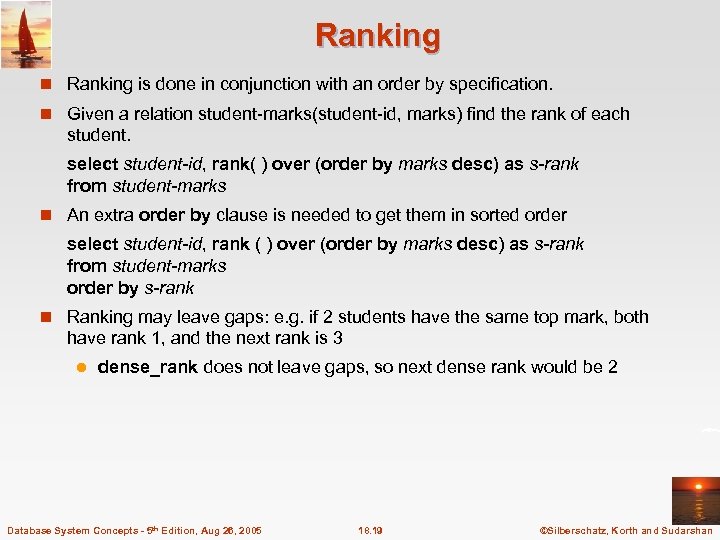
Ranking n Ranking is done in conjunction with an order by specification. n Given a relation student-marks(student-id, marks) find the rank of each student. select student-id, rank( ) over (order by marks desc) as s-rank from student-marks n An extra order by clause is needed to get them in sorted order select student-id, rank ( ) over (order by marks desc) as s-rank from student-marks order by s-rank n Ranking may leave gaps: e. g. if 2 students have the same top mark, both have rank 1, and the next rank is 3 l dense_rank does not leave gaps, so next dense rank would be 2 Database System Concepts - 5 th Edition, Aug 26, 2005 18. 19 ©Silberschatz, Korth and Sudarshan
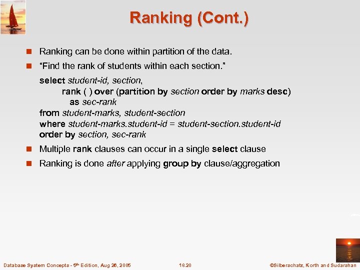
Ranking (Cont. ) n Ranking can be done within partition of the data. n “Find the rank of students within each section. ” select student-id, section, rank ( ) over (partition by section order by marks desc) as sec-rank from student-marks, student-section where student-marks. student-id = student-section. student-id order by section, sec-rank n Multiple rank clauses can occur in a single select clause n Ranking is done after applying group by clause/aggregation Database System Concepts - 5 th Edition, Aug 26, 2005 18. 20 ©Silberschatz, Korth and Sudarshan
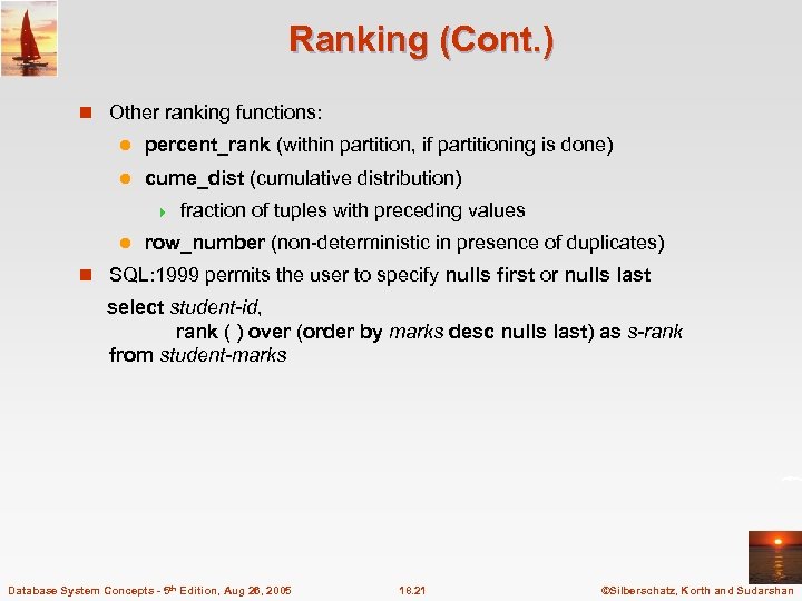
Ranking (Cont. ) n Other ranking functions: l percent_rank (within partition, if partitioning is done) l cume_dist (cumulative distribution) 4 l fraction of tuples with preceding values row_number (non-deterministic in presence of duplicates) n SQL: 1999 permits the user to specify nulls first or nulls last select student-id, rank ( ) over (order by marks desc nulls last) as s-rank from student-marks Database System Concepts - 5 th Edition, Aug 26, 2005 18. 21 ©Silberschatz, Korth and Sudarshan
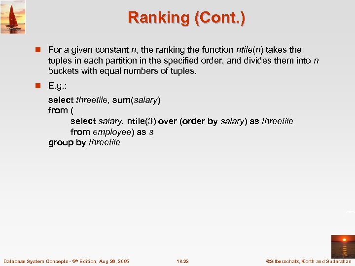
Ranking (Cont. ) n For a given constant n, the ranking the function ntile(n) takes the tuples in each partition in the specified order, and divides them into n buckets with equal numbers of tuples. n E. g. : select threetile, sum(salary) from ( select salary, ntile(3) over (order by salary) as threetile from employee) as s group by threetile Database System Concepts - 5 th Edition, Aug 26, 2005 18. 22 ©Silberschatz, Korth and Sudarshan
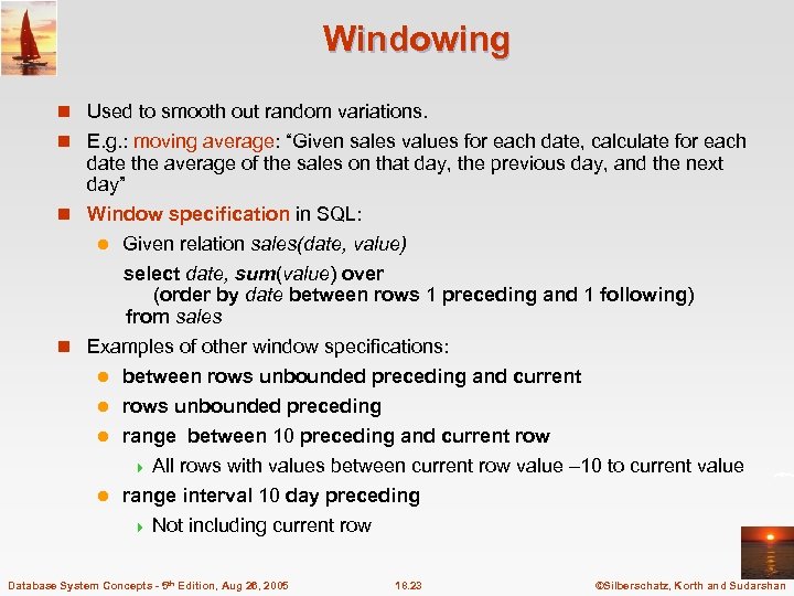
Windowing n Used to smooth out random variations. n E. g. : moving average: “Given sales values for each date, calculate for each date the average of the sales on that day, the previous day, and the next day” n Window specification in SQL: l Given relation sales(date, value) select date, sum(value) over (order by date between rows 1 preceding and 1 following) from sales n Examples of other window specifications: l between rows unbounded preceding and current rows unbounded preceding l range between 10 preceding and current row 4 All rows with values between current row value – 10 to current value l range interval 10 day preceding 4 Not including current row l Database System Concepts - 5 th Edition, Aug 26, 2005 18. 23 ©Silberschatz, Korth and Sudarshan
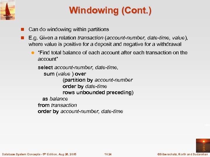
Windowing (Cont. ) n Can do windowing within partitions n E. g. Given a relation transaction (account-number, date-time, value), where value is positive for a deposit and negative for a withdrawal l “Find total balance of each account after each transaction on the account” select account-number, date-time, sum (value ) over (partition by account-number order by date-time rows unbounded preceding) as balance from transaction order by account-number, date-time Database System Concepts - 5 th Edition, Aug 26, 2005 18. 24 ©Silberschatz, Korth and Sudarshan
Data Warehousing n Data sources often store only current data, not historical data n Corporate decision making requires a unified view of all organizational data, including historical data n A data warehouse is a repository (archive) of information gathered from multiple sources, stored under a unified schema, at a single site l Greatly simplifies querying, permits study of historical trends l Shifts decision support query load away from transaction processing systems Database System Concepts - 5 th Edition, Aug 26, 2005 18. 25 ©Silberschatz, Korth and Sudarshan
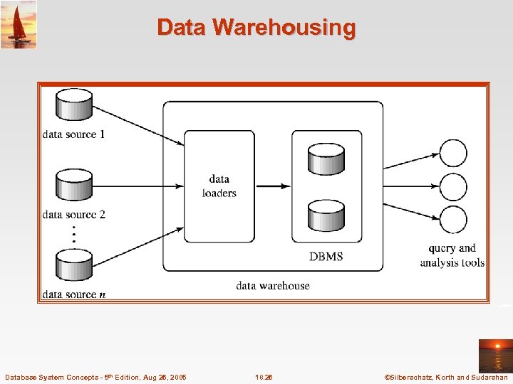
Data Warehousing Database System Concepts - 5 th Edition, Aug 26, 2005 18. 26 ©Silberschatz, Korth and Sudarshan
Design Issues n When and how to gather data l Source driven architecture: data sources transmit new information to warehouse, either continuously or periodically (e. g. at night) l Destination driven architecture: warehouse periodically requests new information from data sources l Keeping warehouse exactly synchronized with data sources (e. g. using two-phase commit) is too expensive 4 Usually OK to have slightly out-of-date data at warehouse 4 Data/updates are periodically downloaded form online transaction processing (OLTP) systems. n What schema to use l Schema integration Database System Concepts - 5 th Edition, Aug 26, 2005 18. 27 ©Silberschatz, Korth and Sudarshan
More Warehouse Design Issues n Data cleansing l E. g. correct mistakes in addresses (misspellings, zip code errors) l Merge address lists from different sources and purge duplicates n How to propagate updates l Warehouse schema may be a (materialized) view of schema from data sources n What data to summarize l Raw data may be too large to store on-line l Aggregate values (totals/subtotals) often suffice l Queries on raw data can often be transformed by query optimizer to use aggregate values Database System Concepts - 5 th Edition, Aug 26, 2005 18. 28 ©Silberschatz, Korth and Sudarshan
Warehouse Schemas n Dimension values are usually encoded using small integers and mapped to full values via dimension tables n Resultant schema is called a star schema l More complicated schema structures 4 Snowflake schema: multiple levels of dimension tables 4 Constellation: Database System Concepts - 5 th Edition, Aug 26, 2005 multiple fact tables 18. 29 ©Silberschatz, Korth and Sudarshan
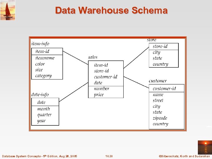
Data Warehouse Schema Database System Concepts - 5 th Edition, Aug 26, 2005 18. 30 ©Silberschatz, Korth and Sudarshan
Data Mining n Data mining is the process of semi-automatically analyzing large databases to find useful patterns n Prediction based on past history l Predict if a credit card applicant poses a good credit risk, based on some attributes (income, job type, age, . . ) and past history l Predict if a pattern of phone calling card usage is likely to be fraudulent n Some examples of prediction mechanisms: l Classification 4 Given a new item whose class is unknown, predict to which class it belongs l Regression formulae 4 Given a set of mappings for an unknown function, predict the function result for a new parameter value Database System Concepts - 5 th Edition, Aug 26, 2005 18. 31 ©Silberschatz, Korth and Sudarshan
Data Mining (Cont. ) n Descriptive Patterns l Associations 4 Find books that are often bought by “similar” customers. If a new such customer buys one such book, suggest the others too. l Associations may be used as a first step in detecting causation 4 E. g. l association between exposure to chemical X and cancer, Clusters 4 E. g. typhoid cases were clustered in an area surrounding a contaminated well 4 Detection of clusters remains important in detecting epidemics Database System Concepts - 5 th Edition, Aug 26, 2005 18. 32 ©Silberschatz, Korth and Sudarshan
Classification Rules n Classification rules help assign new objects to classes. l E. g. , given a new automobile insurance applicant, should he or she be classified as low risk, medium risk or high risk? n Classification rules for above example could use a variety of data, such as educational level, salary, age, etc. l person P, P. degree = masters and P. income > 75, 000 P. credit = excellent l person P, P. degree = bachelors and (P. income 25, 000 and P. income 75, 000) P. credit = good n Rules are not necessarily exact: there may be some misclassifications n Classification rules can be shown compactly as a decision tree. Database System Concepts - 5 th Edition, Aug 26, 2005 18. 33 ©Silberschatz, Korth and Sudarshan
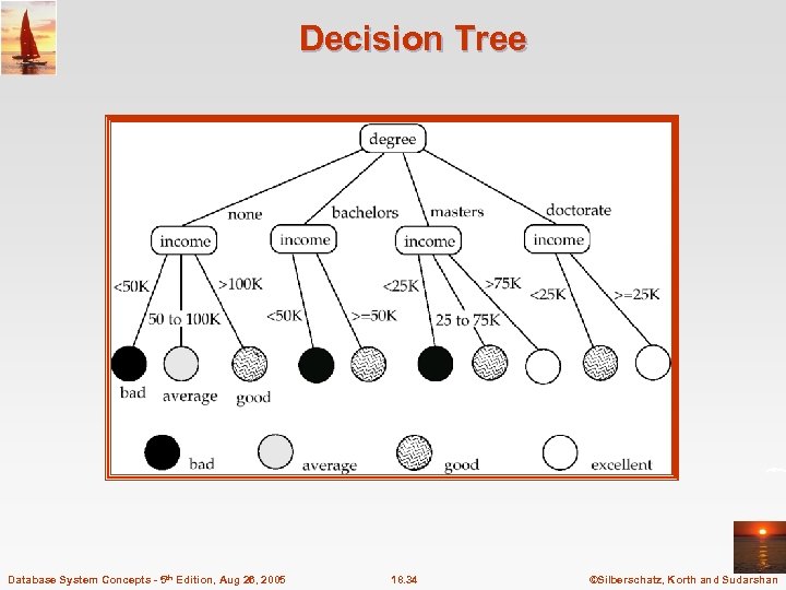
Decision Tree Database System Concepts - 5 th Edition, Aug 26, 2005 18. 34 ©Silberschatz, Korth and Sudarshan
Construction of Decision Trees n Training set: a data sample in which the classification is already known. n Greedy top down generation of decision trees. l Each internal node of the tree partitions the data into groups based on a partitioning attribute, and a partitioning condition for the node l Leaf node: 4 all (or most) of the items at the node belong to the same class, or 4 all attributes have been considered, and no further partitioning is possible. Database System Concepts - 5 th Edition, Aug 26, 2005 18. 35 ©Silberschatz, Korth and Sudarshan
Best Splits n Pick best attributes and conditions on which to partition n The purity of a set S of training instances can be measured quantitatively in several ways. l Notation: number of classes = k, number of instances = |S|, fraction of instances in class i = pi. n The Gini measure of purity is defined as [ k Gini (S) = 1 - p 2 i i- 1 l When all instances are in a single class, the Gini value is 0 l It reaches its maximum (of 1 – 1 /k) if each class the same number of instances. Database System Concepts - 5 th Edition, Aug 26, 2005 18. 36 ©Silberschatz, Korth and Sudarshan
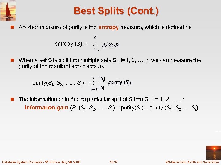
Best Splits (Cont. ) n Another measure of purity is the entropy measure, which is defined as k entropy (S) = – pilog 2 pi i- 1 n When a set S is split into multiple sets Si, I=1, 2, …, r, we can measure the purity of the resultant set of sets as: r purity(S 1, S 2, …. . , Sr) = |Si| i= 1 |S| purity (Si) n The information gain due to particular split of S into Si, i = 1, 2, …. , r Information-gain (S, {S 1, S 2, …. , Sr) = purity(S ) – purity (S 1, S 2, … Sr) Database System Concepts - 5 th Edition, Aug 26, 2005 18. 37 ©Silberschatz, Korth and Sudarshan
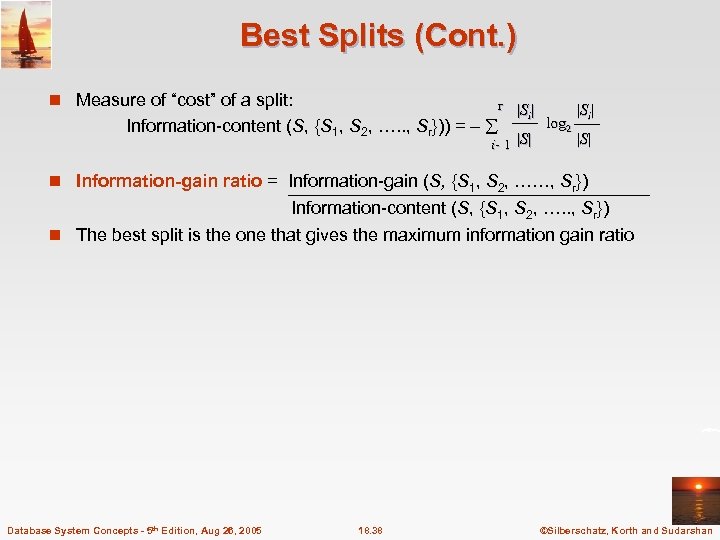
Best Splits (Cont. ) n Measure of “cost” of a split: Information-content (S, {S 1, S 2, …. . , Sr})) = – r |S | i i- 1 |S| log 2 |Si| |S| n Information-gain ratio = Information-gain (S, {S 1, S 2, ……, Sr}) Information-content (S, {S 1, S 2, …. . , Sr}) n The best split is the one that gives the maximum information gain ratio Database System Concepts - 5 th Edition, Aug 26, 2005 18. 38 ©Silberschatz, Korth and Sudarshan
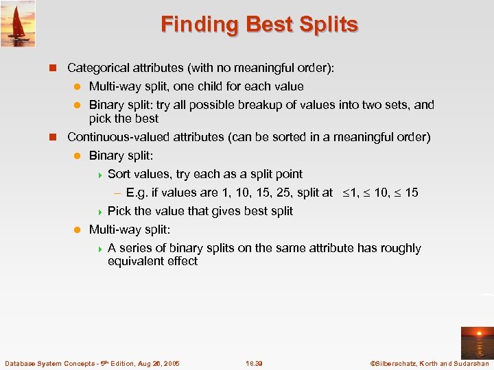
Finding Best Splits n Categorical attributes (with no meaningful order): Multi-way split, one child for each value l Binary split: try all possible breakup of values into two sets, and pick the best n Continuous-valued attributes (can be sorted in a meaningful order) l Binary split: 4 Sort values, try each as a split point – E. g. if values are 1, 10, 15, 25, split at 1, 10, 15 4 Pick the value that gives best split l Multi-way split: l 4 A series of binary splits on the same attribute has roughly equivalent effect Database System Concepts - 5 th Edition, Aug 26, 2005 18. 39 ©Silberschatz, Korth and Sudarshan
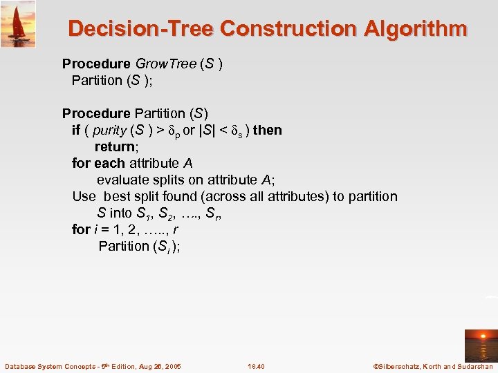
Decision-Tree Construction Algorithm Procedure Grow. Tree (S ) Partition (S ); Procedure Partition (S) if ( purity (S ) > p or |S| < s ) then return; for each attribute A evaluate splits on attribute A; Use best split found (across all attributes) to partition S into S 1, S 2, …. , Sr, for i = 1, 2, …. . , r Partition (Si ); Database System Concepts - 5 th Edition, Aug 26, 2005 18. 40 ©Silberschatz, Korth and Sudarshan
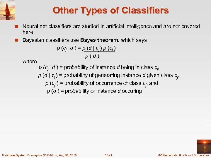
Other Types of Classifiers n Neural net classifiers are studied in artificial intelligence and are not covered here n Bayesian classifiers use Bayes theorem, which says p (cj | d ) = p (d | cj ) p (cj ) p(d) where p (cj | d ) = probability of instance d being in class cj, p (d | cj ) = probability of generating instance d given class cj, p (cj ) = probability of occurrence of class cj, and p (d ) = probability of instance d occuring Database System Concepts - 5 th Edition, Aug 26, 2005 18. 41 ©Silberschatz, Korth and Sudarshan
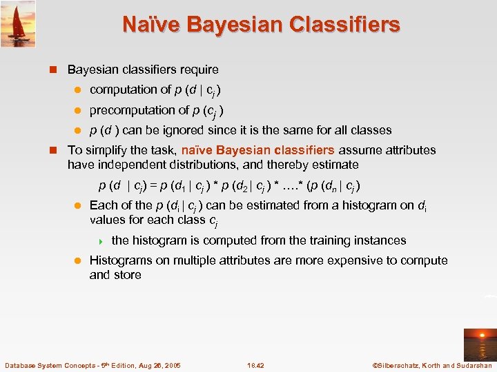
Naïve Bayesian Classifiers n Bayesian classifiers require l computation of p (d | cj ) l precomputation of p (cj ) l p (d ) can be ignored since it is the same for all classes n To simplify the task, naïve Bayesian classifiers assume attributes have independent distributions, and thereby estimate p (d | cj) = p (d 1 | cj ) * p (d 2 | cj ) * …. * (p (dn | cj ) l Each of the p (di | cj ) can be estimated from a histogram on di values for each class cj 4 l the histogram is computed from the training instances Histograms on multiple attributes are more expensive to compute and store Database System Concepts - 5 th Edition, Aug 26, 2005 18. 42 ©Silberschatz, Korth and Sudarshan
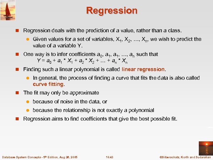
Regression n Regression deals with the prediction of a value, rather than a class. l Given values for a set of variables, X 1, X 2, …, Xn, we wish to predict the value of a variable Y. n One way is to infer coefficients a 0, a 1, …, an such that Y = a 0 + a 1 * X 1 + a 2 * X 2 + … + an * X n n Finding such a linear polynomial is called linear regression. l In general, the process of finding a curve that fits the data is also called curve fitting. n The fit may only be approximate l because of noise in the data, or l because the relationship is not exactly a polynomial n Regression aims to find coefficients that give the best possible fit. Database System Concepts - 5 th Edition, Aug 26, 2005 18. 43 ©Silberschatz, Korth and Sudarshan
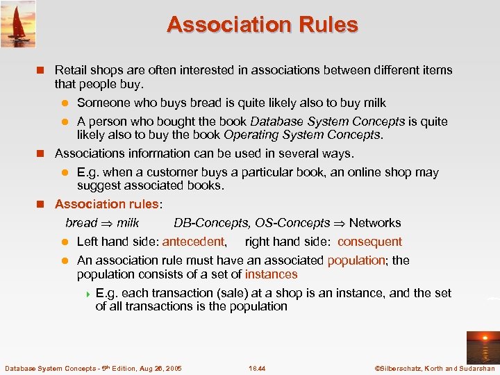
Association Rules n Retail shops are often interested in associations between different items that people buy. l Someone who buys bread is quite likely also to buy milk l A person who bought the book Database System Concepts is quite likely also to buy the book Operating System Concepts. n Associations information can be used in several ways. l E. g. when a customer buys a particular book, an online shop may suggest associated books. n Association rules: bread milk DB-Concepts, OS-Concepts Networks Left hand side: antecedent, right hand side: consequent l An association rule must have an associated population; the population consists of a set of instances 4 E. g. each transaction (sale) at a shop is an instance, and the set of all transactions is the population l Database System Concepts - 5 th Edition, Aug 26, 2005 18. 44 ©Silberschatz, Korth and Sudarshan
Association Rules (Cont. ) n Rules have an associated support, as well as an associated confidence. n Support is a measure of what fraction of the population satisfies both the antecedent and the consequent of the rule. l E. g. suppose only 0. 001 percent of all purchases include milk and screwdrivers. The support for the rule is milk screwdrivers is low. n Confidence is a measure of how often the consequent is true when the antecedent is true. l E. g. the rule bread milk has a confidence of 80 percent if 80 percent of the purchases that include bread also include milk. Database System Concepts - 5 th Edition, Aug 26, 2005 18. 45 ©Silberschatz, Korth and Sudarshan
Finding Association Rules n We are generally only interested in association rules with reasonably high support (e. g. support of 2% or greater) n Naïve algorithm 1. Consider all possible sets of relevant items. 2. For each set find its support (i. e. count how many transactions purchase all items in the set). H 3. Large itemsets: sets with sufficiently high support Use large itemsets to generate association rules. 1. From itemset A generate the rule A - {b } b for each b A. 4 Support of rule = support (A). 4 Confidence of rule = support (A ) / support (A - {b }) Database System Concepts - 5 th Edition, Aug 26, 2005 18. 46 ©Silberschatz, Korth and Sudarshan
Finding Support n Determine support of itemsets via a single pass on set of transactions l Large itemsets: sets with a high count at the end of the pass n If memory not enough to hold all counts for all itemsets use multiple passes, considering only some itemsets in each pass. n Optimization: Once an itemset is eliminated because its count (support) is too small none of its supersets needs to be considered. n The a priori technique to find large itemsets: l Pass 1: count support of all sets with just 1 item. Eliminate those items with low support l Pass i: candidates: every set of i items such that all its i-1 item subsets are large 4 Count 4 Stop support of all candidates if there are no candidates Database System Concepts - 5 th Edition, Aug 26, 2005 18. 47 ©Silberschatz, Korth and Sudarshan
Other Types of Associations n Basic association rules have several limitations n Deviations from the expected probability are more interesting E. g. if many people purchase bread, and many people purchase cereal, quite a few would be expected to purchase both l We are interested in positive as well as negative correlations between sets of items 4 Positive correlation: co-occurrence is higher than predicted 4 Negative correlation: co-occurrence is lower than predicted n Sequence associations / correlations l E. g. whenever bonds go up, stock prices go down in 2 days l n Deviations from temporal patterns E. g. deviation from a steady growth l E. g. sales of winter wear go down in summer 4 Not surprising, part of a known pattern. 4 Look for deviation from value predicted using past patterns l Database System Concepts - 5 th Edition, Aug 26, 2005 18. 48 ©Silberschatz, Korth and Sudarshan
Clustering n Clustering: Intuitively, finding clusters of points in the given data such that similar points lie in the same cluster n Can be formalized using distance metrics in several ways l Group points into k sets (for a given k) such that the average distance of points from the centroid of their assigned group is minimized 4 Centroid: point defined by taking average of coordinates in each dimension. l Another metric: minimize average distance between every pair of points in a cluster n Has been studied extensively in statistics, but on small data sets l Data mining systems aim at clustering techniques that can handle very large data sets l E. g. the Birch clustering algorithm (more shortly) Database System Concepts - 5 th Edition, Aug 26, 2005 18. 49 ©Silberschatz, Korth and Sudarshan
Hierarchical Clustering n Example from biological classification l (the word classification here does not mean a prediction mechanism) chordata mammalia leopards humans reptilia snakes crocodiles n Other examples: Internet directory systems (e. g. Yahoo, more on this later) n Agglomerative clustering algorithms l Build small clusters, then cluster small clusters into bigger clusters, and so on n Divisive clustering algorithms l Start with all items in a single cluster, repeatedly refine (break) clusters into smaller ones Database System Concepts - 5 th Edition, Aug 26, 2005 18. 50 ©Silberschatz, Korth and Sudarshan
Clustering Algorithms n Clustering algorithms have been designed to handle very large datasets n E. g. the Birch algorithm l Main idea: use an in-memory R-tree to store points that are being clustered l Insert points one at a time into the R-tree, merging a new point with an existing cluster if is less than some distance away l If there are more leaf nodes than fit in memory, merge existing clusters that are close to each other l At the end of first pass we get a large number of clusters at the leaves of the R-tree 4 Merge clusters to reduce the number of clusters Database System Concepts - 5 th Edition, Aug 26, 2005 18. 51 ©Silberschatz, Korth and Sudarshan
Collaborative Filtering n Goal: predict what movies/books/… a person may be interested in, on the basis of l Past preferences of the person l Other people with similar past preferences l The preferences of such people for a new movie/book/… n One approach based on repeated clustering l Cluster people on the basis of preferences for movies l Then cluster movies on the basis of being liked by the same clusters of people l Again cluster people based on their preferences for (the newly created clusters of) movies l Repeat above till equilibrium n Above problem is an instance of collaborative filtering, where users collaborate in the task of filtering information to find information of interest Database System Concepts - 5 th Edition, Aug 26, 2005 18. 52 ©Silberschatz, Korth and Sudarshan
Other Types of Mining n Text mining: application of data mining to textual documents l cluster Web pages to find related pages l cluster pages a user has visited to organize their visit history l classify Web pages automatically into a Web directory n Data visualization systems help users examine large volumes of data and detect patterns visually l Can visually encode large amounts of information on a single screen l Humans are very good a detecting visual patterns Database System Concepts - 5 th Edition, Aug 26, 2005 18. 53 ©Silberschatz, Korth and Sudarshan
b85155f296e26efb7f864d2fc7449b75.ppt