Chapter 17 Output and the Exchange Rate in

Chapter 17 Output and the Exchange Rate in the Short Run

Preview • Determinants of aggregate demand in the short run • A short-run model of output markets – DD schedule • A short-run model of asset markets – AA schedule • A short-run model for both output markets and asset markets (AA and DD schedules) • Effects of temporary and permanent changes in monetary and fiscal policies • Adjustment of the current account over time • Liquidity trap Copyright © 2015 Pearson Education, Inc. All rights reserved. 17 -2

Introduction • Long-run models are useful when all prices of inputs and outputs have time to adjust. • In the short run, some prices of inputs and outputs may not have time to adjust. • The reasons for this include: long-term labor contracts, costs of adjustment (menu costs), or imperfect information about willingness of customers to pay at different prices. Copyright © 2015 Pearson Education, Inc. All rights reserved. 17 -3

Introduction • In previous chapters we examined the relation between output, inflation, interest rates, and exchange rates; assuming that the level of output was an exogenous factor. • This chapter builds on the short-run and long-run models of exchange rates to explain how output interacts with exchange rates in the short run. – This model shows how macroeconomic policies can affect production, employment, and the current account. Copyright © 2015 Pearson Education, Inc. All rights reserved. 17 -4

Determinants of Aggregate Demand • Aggregate demand is the aggregate amount of goods and services that individuals and institutions are willing to buy: 1. consumption expenditure 2. investment expenditure 3. government purchases 4. net expenditure by foreigners: the current account Copyright © 2015 Pearson Education, Inc. All rights reserved. 17 -5

Determinants of Consumption Expenditures • Disposable income: income from production (Y) minus taxes (T). – More disposable income means more consumption expenditure, but consumption typically increases less than the amount that disposable income increases. • Real interest rates may influence the amount of saving and spending on consumption goods, but we assume that they are relatively unimportant here. • Wealth may also influence consumption expenditure, but we assume that it is relatively unimportant here. Copyright © 2015 Pearson Education, Inc. All rights reserved. 17 -6

How Real Exchange Rate Changes Affect the Current Account • The current account measures the value of exports relative to the value of imports: CA ≈ EX – IM. • When the real exchange rate EP*/P rises (depreciates), the foreign prices rise relative to the domestic prices. 1. The volume of exports that are bought by foreigners rises. 2. The volume of imports that are bought by domestic residents falls. 3. The value of imports in terms of domestic products rises: the value/price of imports rises, since foreign products are more valuable/expensive. Copyright © 2015 Pearson Education, Inc. All rights reserved. 17 -7

How Real Exchange Rate Changes Affect the Current Account • If the volumes of imports and exports do not change much, the value effect may dominate the volume effect when the real exchange rate changes. – For example, contract obligations to buy fixed amounts of products may cause the volume effect to be small. • However, evidence indicates that for most countries the volume effect dominates the value effect after one year or less. • Let’s assume for now that a real depreciation leads to an increase in the current account: the volume effect dominates the value effect. Copyright © 2015 Pearson Education, Inc. All rights reserved. 17 -8

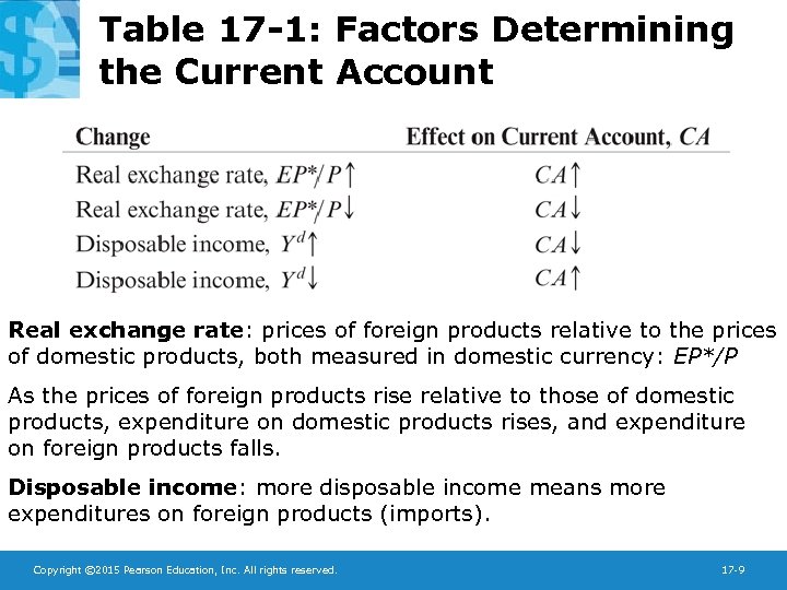Table 17 -1: Factors Determining the Current Account Real exchange rate: prices of foreign products relative to the prices of domestic products, both measured in domestic currency: EP*/P As the prices of foreign products rise relative to those of domestic products, expenditure on domestic products rises, and expenditure on foreign products falls. Disposable income: more disposable income means more expenditures on foreign products (imports). Copyright © 2015 Pearson Education, Inc. All rights reserved. 17 -9

Determinants of Aggregate Demand • For simplicity, we assume that exogenous political factors determine government purchases G and the level of taxes T. – A more complicated model may assume that government purchases and taxes depend on a business cycle. • For simplicity, we currently assume that investment expenditure I is determined by exogenous business decisions. – A more complicated model shows that investment depends on the cost of spending or borrowing to finance investment: the interest rate. Copyright © 2015 Pearson Education, Inc. All rights reserved. 17 -10

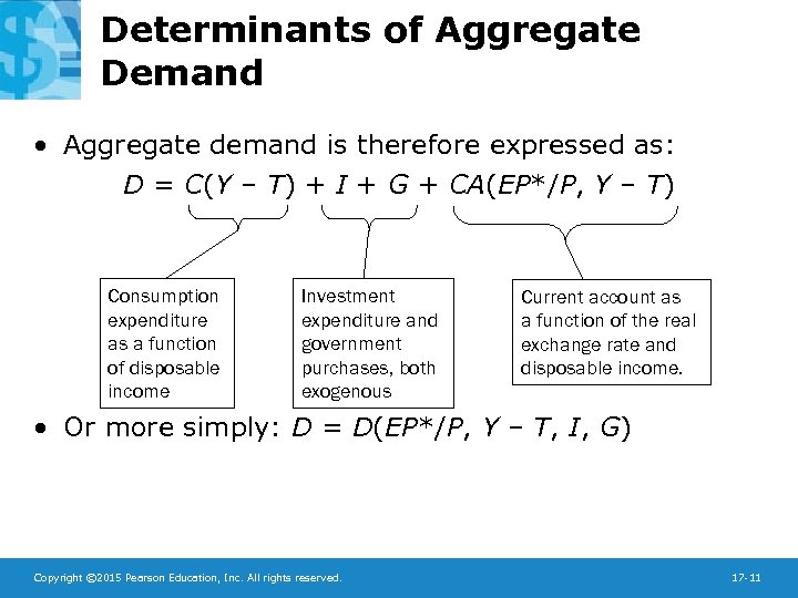Determinants of Aggregate Demand • Aggregate demand is therefore expressed as: D = C(Y – T) + I + G + CA(EP*/P, Y – T) Consumption expenditure as a function of disposable income Investment expenditure and government purchases, both exogenous Current account as a function of the real exchange rate and disposable income. • Or more simply: D = D(EP*/P, Y – T, I, G) Copyright © 2015 Pearson Education, Inc. All rights reserved. 17 -11

Determinants of Aggregate Demand • Real exchange rate: an increase in the real exchange rate (real depreciation) increases the current account, and therefore increases aggregate demand of domestic products. • Disposable income: an increase in the disposable income increases consumption expenditure, but decreases the current account. – Since consumption expenditure is usually greater than expenditure on foreign products, the first effect dominates the second effect. – As income increases for a given level of taxes, aggregate consumption expenditure and aggregate demand increase by less than income. Copyright © 2015 Pearson Education, Inc. All rights reserved. 17 -12

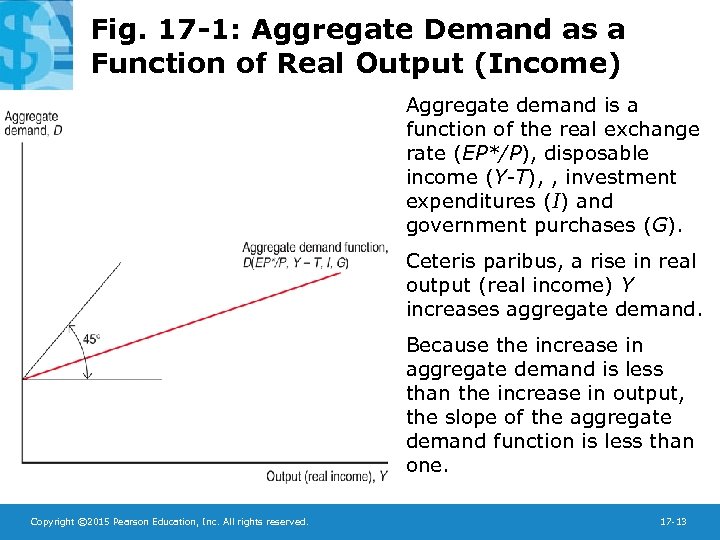Fig. 17 -1: Aggregate Demand as a Function of Real Output (Income) Aggregate demand is a function of the real exchange rate (EP*/P), disposable income (Y-T), , investment expenditures (I) and government purchases (G). Ceteris paribus, a rise in real output (real income) Y increases aggregate demand. Because the increase in aggregate demand is less than the increase in output, the slope of the aggregate demand function is less than one. Copyright © 2015 Pearson Education, Inc. All rights reserved. 17 -13

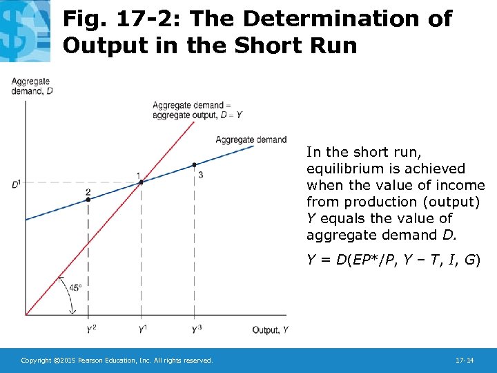Fig. 17 -2: The Determination of Output in the Short Run In the short run, equilibrium is achieved when the value of income from production (output) Y equals the value of aggregate demand D. Y = D(EP*/P, Y – T, I, G) Copyright © 2015 Pearson Education, Inc. All rights reserved. 17 -14

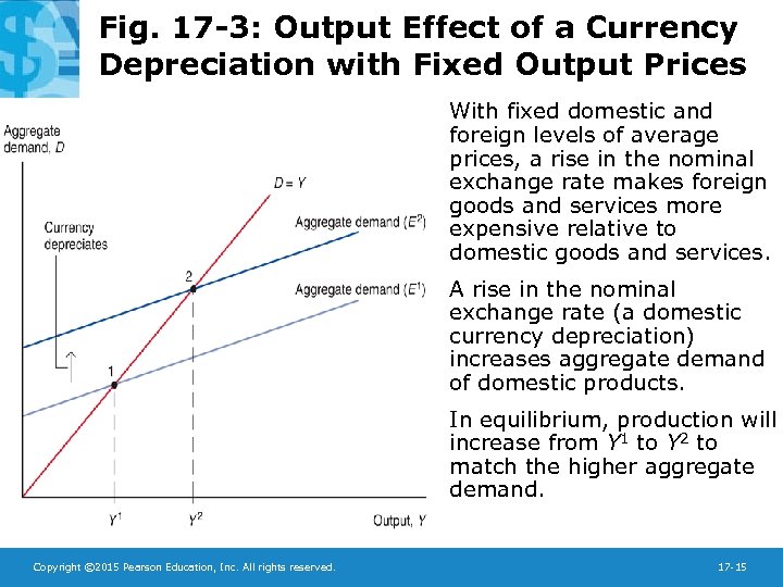Fig. 17 -3: Output Effect of a Currency Depreciation with Fixed Output Prices With fixed domestic and foreign levels of average prices, a rise in the nominal exchange rate makes foreign goods and services more expensive relative to domestic goods and services. A rise in the nominal exchange rate (a domestic currency depreciation) increases aggregate demand of domestic products. In equilibrium, production will increase from Y 1 to Y 2 to match the higher aggregate demand. Copyright © 2015 Pearson Education, Inc. All rights reserved. 17 -15

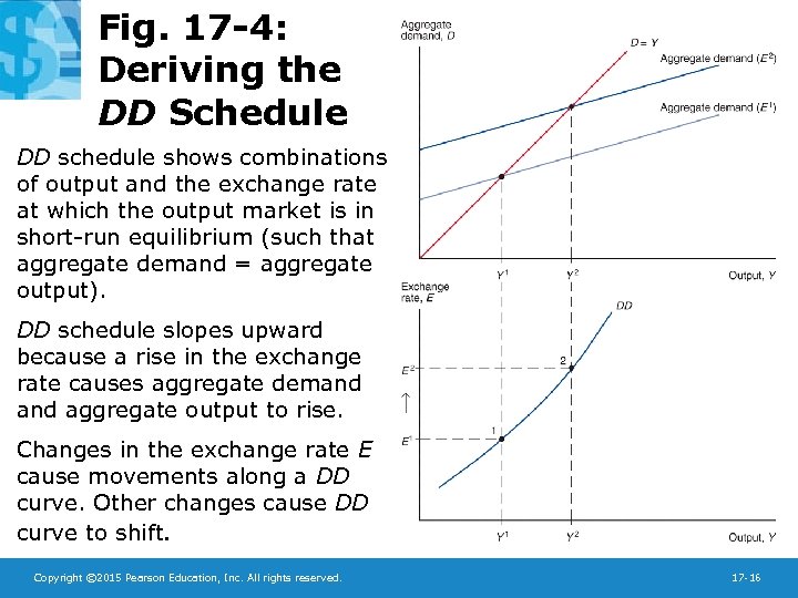Fig. 17 -4: Deriving the DD Schedule DD schedule shows combinations of output and the exchange rate at which the output market is in short-run equilibrium (such that aggregate demand = aggregate output). DD schedule slopes upward because a rise in the exchange rate causes aggregate demand aggregate output to rise. Changes in the exchange rate E cause movements along a DD curve. Other changes cause DD curve to shift. Copyright © 2015 Pearson Education, Inc. All rights reserved. 17 -16

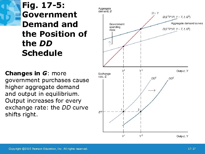Fig. 17 -5: Government Demand the Position of the DD Schedule Changes in G: more government purchases cause higher aggregate demand output in equilibrium. Output increases for every exchange rate: the DD curve shifts right. Copyright © 2015 Pearson Education, Inc. All rights reserved. 17 -17

Shifting the DD Curve • Changes in G: more government purchases cause higher aggregate demand output in equilibrium. Output increases for every exchange rate: the DD curve shifts right. • Changes in T: lower taxes generally increase consumption expenditure, increasing aggregate demand output in equilibrium for every exchange rate: the DD curve shifts right. • Changes in I: higher investment expenditure is represented by shifting the DD curve right. Copyright © 2015 Pearson Education, Inc. All rights reserved. 17 -18

Shifting the DD Curve • Changes in P relative to P*: lower domestic prices relative to foreign prices are represented by shifting the DD curve right. • Changes in C: willingness to consume more and save less is represented by shifting the DD curve right. • Changes in demand of domestic goods relative to foreign goods: willingness to consume more domestic goods relative to foreign goods is represented by shifting the DD curve right. Copyright © 2015 Pearson Education, Inc. All rights reserved. 17 -19

Short-Run Equilibrium in Asset Markets • We consider two sets of asset markets: 1. Foreign exchange markets – interest parity represents equilibrium: R = R* + (Ee – E)/E 2. Money market – Equilibrium occurs when the quantity of real monetary assets supplied matches the quantity of real monetary assets demanded: Ms/P = L(R, Y) – A rise in income from production causes the demand of real monetary assets to increase. – An increase in the interest rate lowers the demand for real money balances, as it rises the opportunity costs of holdnig money. Copyright © 2015 Pearson Education, Inc. All rights reserved. 17 -20

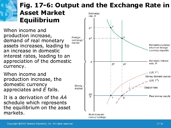Fig. 17 -6: Output and the Exchange Rate in Asset Market Equilibrium When income and production increase, demand of real monetary assets increases, leading to an increase in domestic interest rates, leading to an appreciation of the domestic currency. When income and production increase, the domestic currency appreciates and E falls. It is a derivation of the AA schedule which represents the equilibrium on the asset markets. Copyright © 2015 Pearson Education, Inc. All rights reserved. 17 -21

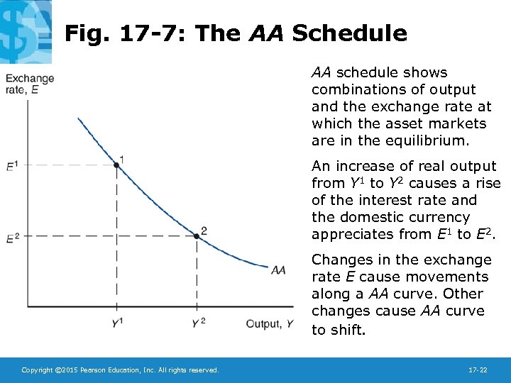Fig. 17 -7: The AA Schedule AA schedule shows combinations of output and the exchange rate at which the asset markets are in the equilibrium. An increase of real output from Y 1 to Y 2 causes a rise of the interest rate and the domestic currency appreciates from E 1 to E 2. Changes in the exchange rate E cause movements along a AA curve. Other changes cause AA curve to shift. Copyright © 2015 Pearson Education, Inc. All rights reserved. 17 -22

Shifting the AA Curve • Changes in Ms: an increase in the money supply reduces interest rates in the short run, causing the domestic currency to depreciate (a rise in E) for every Y: the AA curve shifts up (right). • Changes in P: An increase in the level of average domestic prices decreases the supply of real monetary assets, increasing interest rates, causing the domestic currency to appreciate (a fall in E): the AA curve shifts down (left). • Changes in R*: An increase in the foreign interest rates makes foreign currency deposits more attractive, leading to a depreciation of the domestic currency (a rise in E): the AA curve shifts up (right). Copyright © 2015 Pearson Education, Inc. All rights reserved. 17 -23

Shifting the AA Curve • Changes in the demand of real monetary assets: if domestic residents are willing to hold a lower amount of real money assets and more non-monetary assets, interest rates on nonmonetary assets would fall, leading to a depreciation of the domestic currency (a rise in E): the AA curve shifts up (right). • Changes in Ee: if market participants expect the domestic currency to depreciate in the future, foreign currency deposits become more attractive, causing the domestic currency to depreciate (a rise in E): the AA curve shifts up (right). Copyright © 2015 Pearson Education, Inc. All rights reserved. 17 -24

Putting the Pieces Together: the DD and AA Curves • A short-run equilibrium means a nominal exchange rate and level of output such that 1. equilibrium in the output markets holds: aggregate demand equals aggregate output. 2. equilibrium in the foreign exchange markets holds: interest parity holds. 3. equilibrium in the money market holds: the quantity of real monetary assets supplied equals the quantity of real monetary assets demanded. Copyright © 2015 Pearson Education, Inc. All rights reserved. 17 -25

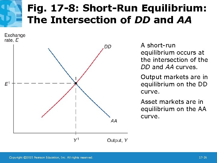Fig. 17 -8: Short-Run Equilibrium: The Intersection of DD and AA A short-run equilibrium occurs at the intersection of the DD and AA curves. Output markets are in equilibrium on the DD curve. Asset markets are in equilibrium on the AA curve. Copyright © 2015 Pearson Education, Inc. All rights reserved. 17 -26

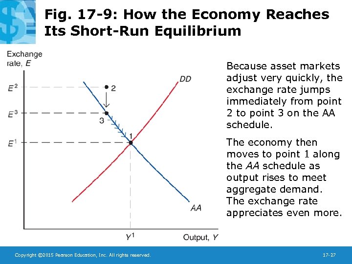Fig. 17 -9: How the Economy Reaches Its Short-Run Equilibrium Because asset markets adjust very quickly, the exchange rate jumps immediately from point 2 to point 3 on the AA schedule. The economy then moves to point 1 along the AA schedule as output rises to meet aggregate demand. The exchange rate appreciates even more. Copyright © 2015 Pearson Education, Inc. All rights reserved. 17 -27

Macroeconomic Stabilization Policies • Monetary policy: policy in which the central bank influences the supply of monetary assets. – Monetary policy is assumed to affect asset markets first. • Fiscal policy: policy in which governments influence the amount of government purchases and taxes. – Fiscal policy is assumed to affect aggregate demand output first. • Temporary policy changes are expected to be reversed in the near future and thus do not affect expectations about exchange rates in the long run. • Permanent policy changes alter the expectations of people about exchange rates in the long run. Copyright © 2015 Pearson Education, Inc. All rights reserved. 17 -28

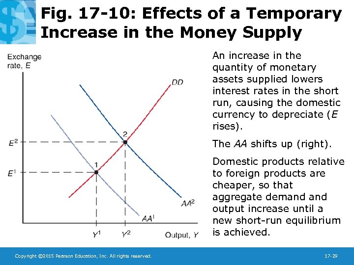Fig. 17 -10: Effects of a Temporary Increase in the Money Supply An increase in the quantity of monetary assets supplied lowers interest rates in the short run, causing the domestic currency to depreciate (E rises). The AA shifts up (right). Domestic products relative to foreign products are cheaper, so that aggregate demand output increase until a new short-run equilibrium is achieved. Copyright © 2015 Pearson Education, Inc. All rights reserved. 17 -29

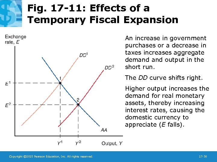Fig. 17 -11: Effects of a Temporary Fiscal Expansion An increase in government purchases or a decrease in taxes increases aggregate demand output in the short run. The DD curve shifts right. Higher output increases the demand for real monetary assets, thereby increasing interest rates, causing the domestic currency to appreciate (E falls). Copyright © 2015 Pearson Education, Inc. All rights reserved. 17 -30

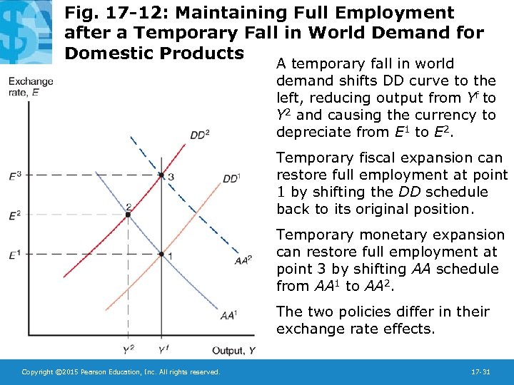Fig. 17 -12: Maintaining Full Employment after a Temporary Fall in World Demand for Domestic Products A temporary fall in world demand shifts DD curve to the left, reducing output from Yf to Y 2 and causing the currency to depreciate from E 1 to E 2. Temporary fiscal expansion can restore full employment at point 1 by shifting the DD schedule back to its original position. Temporary monetary expansion can restore full employment at point 3 by shifting AA schedule from AA 1 to AA 2. The two policies differ in their exchange rate effects. Copyright © 2015 Pearson Education, Inc. All rights reserved. 17 -31

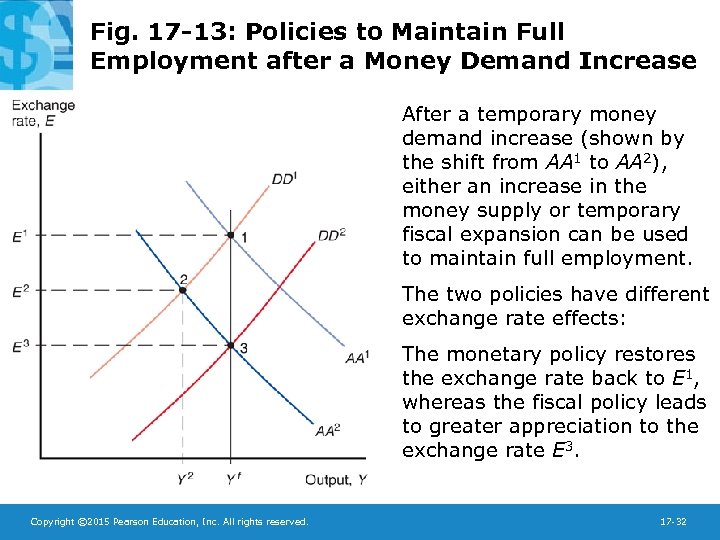Fig. 17 -13: Policies to Maintain Full Employment after a Money Demand Increase After a temporary money demand increase (shown by the shift from AA 1 to AA 2), either an increase in the money supply or temporary fiscal expansion can be used to maintain full employment. The two policies have different exchange rate effects: The monetary policy restores the exchange rate back to E 1, whereas the fiscal policy leads to greater appreciation to the exchange rate E 3. Copyright © 2015 Pearson Education, Inc. All rights reserved. 17 -32

Policies to Maintain Full Employment • Policies to maintain full employment may seem easy in theory, but are hard in practice. 1. Economic data are difficult to measure, they are available with lags, and they are not very reliable. 2. In practice, it is hard to find whether a disturbance to the economy originates in the output or the asset markets. Copyright © 2015 Pearson Education, Inc. All rights reserved. 17 -33

Policies to Maintain Full Employment 3. Changes in policies take time to be implemented and to affect the economy. – Policies may affect the economy after the effects of an economic change have dissipated and therefore this policy may destabilize the economy. 4. Policies are sometimes influenced by political or bureaucratic interests. Copyright © 2015 Pearson Education, Inc. All rights reserved. 17 -34

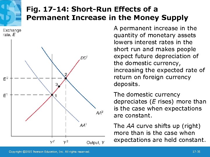Fig. 17 -14: Short-Run Effects of a Permanent Increase in the Money Supply A permanent increase in the quantity of monetary assets lowers interest rates in the short run and makes people expect future depreciation of the domestic currency, increasing the expected rate of return on foreign currency deposits. The domestic currency depreciates (E rises) more than is the case when expectations are constant. The AA curve shifts up (right) more than is the case when expectations are held constant. Copyright © 2015 Pearson Education, Inc. All rights reserved. 17 -35

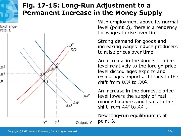Fig. 17 -15: Long-Run Adjustment to a Permanent Increase in the Money Supply With employment above its normal level (point 2), there is a tendency for wages to rise over time. Strong demand for goods and increasing wages induce producers to raise prices over time. An increase in the domestic price level relatively to the foreign price level discourages exports and encourages imports. It leads to the shift from DD 1 to DD 2. An increase in the domestic price level lowers the supply of real money balances and leads to the shift from AA 2 to AA 3. New long-run equilibrium is at point 3. Copyright © 2015 Pearson Education, Inc. All rights reserved. 17 -36

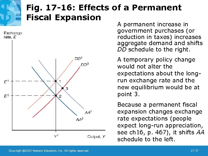Fig. 17 -16: Effects of a Permanent Fiscal Expansion A permanent increase in government purchases (or reduction in taxes) increases aggregate demand shifts DD schedule to the right. A temporary policy change would not alter the expectations about the longrun exchange rate and the new equilibrium would be at point 3. Because a permanent fiscal expansion changes exchange rate expectations (people expect long-run appreciation, see ch 16, p. 467), it shifts AA schedule to the left. Copyright © 2015 Pearson Education, Inc. All rights reserved. 17 -37

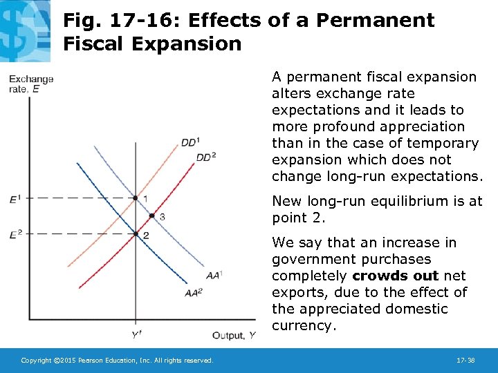Fig. 17 -16: Effects of a Permanent Fiscal Expansion A permanent fiscal expansion alters exchange rate expectations and it leads to more profound appreciation than in the case of temporary expansion which does not change long-run expectations. New long-run equilibrium is at point 2. We say that an increase in government purchases completely crowds out net exports, due to the effect of the appreciated domestic currency. Copyright © 2015 Pearson Education, Inc. All rights reserved. 17 -38

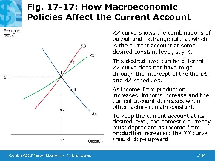Fig. 17 -17: How Macroeconomic Policies Affect the Current Account XX curve shows the combinations of output and exchange rate at which is the current account at some desired constant level, say X. This desired level can be different, XX curve does not have to go through the intercept of the DD and AA schedules. As income from production increases, imports increase and the current account decreases when other factors remain constant. To keep the current account at its desired level, the domestic currency must depreciate as income from production increases: the XX curve should slope upward. Copyright © 2015 Pearson Education, Inc. All rights reserved. 17 -39

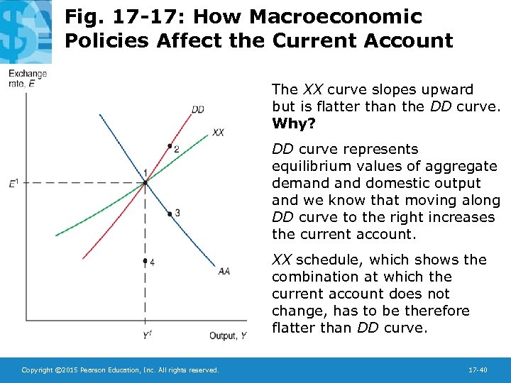Fig. 17 -17: How Macroeconomic Policies Affect the Current Account The XX curve slopes upward but is flatter than the DD curve. Why? DD curve represents equilibrium values of aggregate demand domestic output and we know that moving along DD curve to the right increases the current account. XX schedule, which shows the combination at which the current account does not change, has to be therefore flatter than DD curve. Copyright © 2015 Pearson Education, Inc. All rights reserved. 17 -40

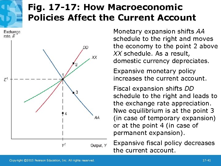Fig. 17 -17: How Macroeconomic Policies Affect the Current Account Monetary expansion shifts AA schedule to the right and moves the economy to the point 2 above XX schedule. As a result, domestic currency depreciates. Expansive monetary policy increases the current account. Fiscal expansion shifts DD schedule to the right and leads to the exchange rate appreciation. Nwe equilibrium is at the point 3 (in case of temporary expansion) or at the point 4 (in case of permanent expansion). Expansive fiscal policy decreases the current account. Copyright © 2015 Pearson Education, Inc. All rights reserved. 17 -41

Macroeconomic Policies and the Current Account • The assumption of DD-AA model is that (ceteris paribus) a real depreciation of exchange rate increases the current account, and vice versa. • In practice, it need not be the case in the short run, due to the value effect, see the next slide. Copyright © 2015 Pearson Education, Inc. All rights reserved. 17 -42

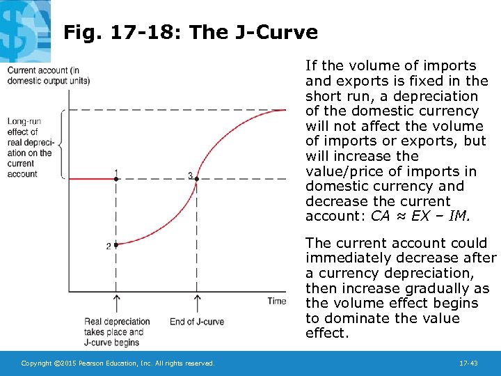Fig. 17 -18: The J-Curve If the volume of imports and exports is fixed in the short run, a depreciation of the domestic currency will not affect the volume of imports or exports, but will increase the value/price of imports in domestic currency and decrease the current account: CA ≈ EX – IM. The current account could immediately decrease after a currency depreciation, then increase gradually as the volume effect begins to dominate the value effect. Copyright © 2015 Pearson Education, Inc. All rights reserved. 17 -43

Value Effect, Volume Effect, and the J-Curve • Pass-through from the exchange rate to import prices measures the percentage by which import prices change when the value of the domestic currency changes by 1%. • In the DD-AA model, the pass-through rate is 1: import prices in domestic currency exactly match a depreciation of the domestic currency. • In reality, pass-through may be less than 1 due to price discrimination in different countries. – Firms that set prices may decide not to match changes in the exchange rate with changes in prices of foreign products denominated in domestic currency. Copyright © 2015 Pearson Education, Inc. All rights reserved. 17 -44

Value Effect, Volume Effect, and the J-Curve • If prices of foreign products in domestic currency do not change much because of a pass-through rate less than 1, then – the value of imports will not rise much after a domestic currency depreciation, and the current account will not fall much, making the J-curve effect smaller. – the volume of imports and exports will not adjust much over time, since domestic currency prices do not change much. • Pass-through of less than 1 dampens the effect of depreciation or appreciation on the current account. Copyright © 2015 Pearson Education, Inc. All rights reserved. 17 -45

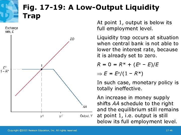Fig. 17 -19: A Low-Output Liquidity Trap At point 1, output is below its full employment level. Liquidity trap occurs at situation when central bank is not able to lower the interest rate, because it is already set to zero. R = 0 = R* + (Ee – E)/E Þ E = Ee/(1 – R*) In such case, monetary policy is totally ineffective. An increase in money supply shifts AA schedule to the right and the equilibrium still remains at point 1, i. e. output is still below its full employment level. Copyright © 2015 Pearson Education, Inc. All rights reserved. 17 -46

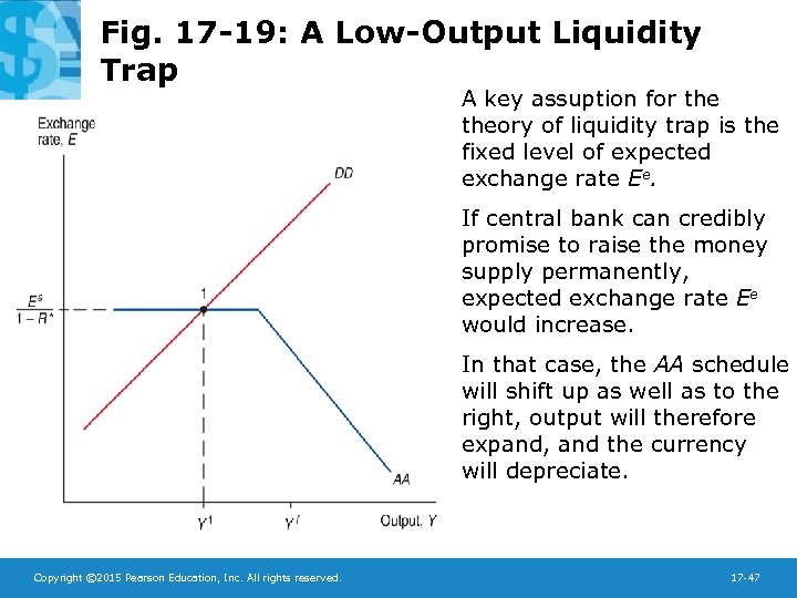Fig. 17 -19: A Low-Output Liquidity Trap A key assuption for theory of liquidity trap is the fixed level of expected exchange rate Ee. If central bank can credibly promise to raise the money supply permanently, expected exchange rate Ee would increase. In that case, the AA schedule will shift up as well as to the right, output will therefore expand, and the currency will depreciate. Copyright © 2015 Pearson Education, Inc. All rights reserved. 17 -47

Summary 1. Aggregate demand is influenced by disposable income and the real exchange rate. 2. The DD curve shows combinations of exchange rates and output where aggregate demand = aggregate output. 3. The AA curve shows combinations of exchange rates and output where the foreign exchange markets and money market are in equilibrium. 4. In the DD-AA model, we assume that a depreciation of the domestic currency leads to an increase in the current account and aggregate demand. – But reality is more complicated, and the J-curve shows that the value effect at first dominates the volume effect. Copyright © 2015 Pearson Education, Inc. All rights reserved. 17 -48

Summary 5. A temporary increase in the money supply is predicted to increase output and depreciate the domestic currency. 6. A permanent increase does both to a larger degree in the short run, but in the long run output returns to its normal level. 7. A temporary increase in government purchases is predicted to increase output and appreciate the domestic currency. 8. A permanent increase in government purchases is predicted to completely crowd out net exports, and therefore to have no effect on output. Copyright © 2015 Pearson Education, Inc. All rights reserved. 17 -49