Chapter 17 Markets with Asymmetric Information Topics

Chapter 17 Markets with Asymmetric Information

Topics to be Discussed l Quality Uncertainty and the Market for Lemons l Market Signaling l Moral Hazard l The Principal-Agent Problem l Managerial Incentives in an Integrated Firm l Asymmetric Information in Labor Markets: Efficiency Wage Theory © 2005 Pearson Education, Inc. Chapter 17 2

Introduction l We can see what happens when some parties know more than others – asymmetric information l Frequently a seller or producer knows more about he quality of the product than the buyer does l Managers know more about costs, competitive position and investment opportunities than firm owners © 2005 Pearson Education, Inc. Chapter 17 3

Quality Uncertainty and the Market for Lemons l Asymmetric information is a situation in which a buyer and a seller possess different information about a transaction m The lack of complete information when purchasing a used car increases the risk of the purchase and lowers the value of the car. m Markets for insurance, financial credit and employment are also characterized by asymmetric information about product quality © 2005 Pearson Education, Inc. Chapter 17 4

The Market for Used Cars l Assume m Two kinds of cars – high quality and low quality m Buyers and sellers can distinguish between the cars m There will be two markets – one for high quality and one for low quality © 2005 Pearson Education, Inc. Chapter 17 5

The Market for Used Cars l High quality market m SH is supply and DH is demand for high quality l Low quality market m SL is supply and DL is demand for low quality l SH is higher than SL because owners of high quality cars need more money to sell them l DH is higher than DL because people are willing to pay more for higher quality © 2005 Pearson Education, Inc. Chapter 17 6

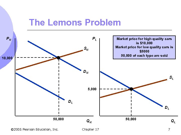The Lemons Problem PH PL SH 10, 000 Market price for high quality cars is $10, 000 Market price for low quality cars is $5000 50, 000 of each type are sold DH SL 5, 000 DL DL 50, 000 © 2005 Pearson Education, Inc. QH Chapter 17 50, 000 QL 7

The Market for Used Cars l Sellers know more about the quality of the used car than the buyer l Initially buyers may think the odds are 50/50 that the car is high quality m Buyers will view all cars as medium quality with demand DM l However, fewer high quality cars (25, 000) and more low quality cars (75, 000) will now be sold l Perceived demand will now shift © 2005 Pearson Education, Inc. Chapter 17 8

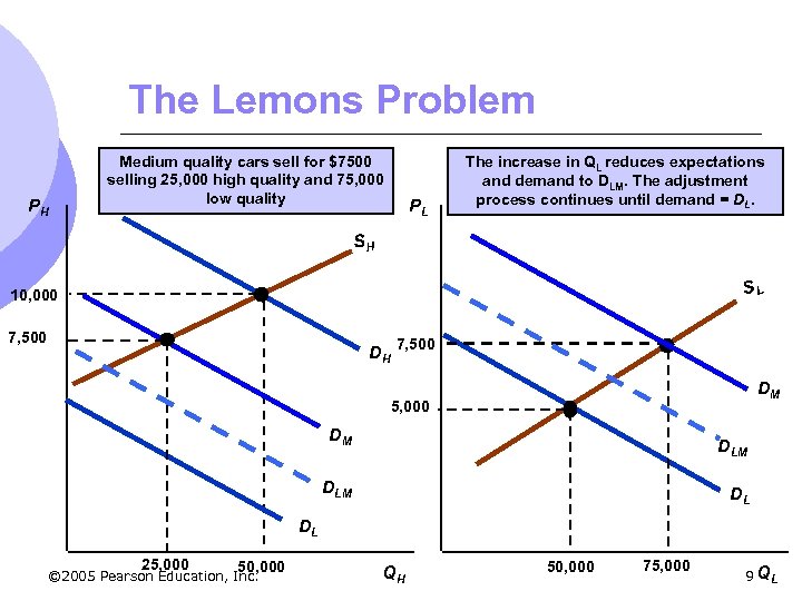The Lemons Problem PH Medium quality cars sell for $7500 selling 25, 000 high quality and 75, 000 low quality PL The increase in QL reduces expectations and demand to DLM. The adjustment process continues until demand = DL. SH SL 10, 000 7, 500 DH 7, 500 DM 5, 000 DM DLM DL DL 25, 000 50, 000 © 2005 Pearson Education, Inc. QH 50, 000 75, 000 9 QL

The Market for Used Cars l With asymmetric information: m Low quality goods drive high quality goods out of the market- the lemons problem. m The market has failed to produce mutually beneficial trade. m Too many low and too few high quality cars are on the market. m Adverse selection occurs; the only cars on the market will be low quality cars. © 2005 Pearson Education, Inc. Chapter 17 10

Market for Insurance l Older individuals have difficulty purchasing health insurance at almost any price l They know more about their health than the insurance company l Because unhealthy people are more likely to want insurance, proportion of unhealthy people in the pool of insured people rises l Price of insurance rises so healthy people with low risk drop out – proportion of unhealthy people rises increasing price more © 2005 Pearson Education, Inc. Chapter 17 11

Market for Insurance l If auto insurance companies are targeting a certain population – males under 25 l They know some of the males have low probability of getting in an accident and some have a high probability l If can’t distinguish among insured, it will base premium on the average experience l Some with low risk will choose not to insure and with raises the accident probability and rates © 2005 Pearson Education, Inc. Chapter 17 12

Market for Insurance l A possible solution to this problem is to pool risks m Health insurance – government takes on role as with Medicare program l Problem of adverse selection is eliminated m Insurance companies will try to avoid risk by offering group health insurance policies at places of employment and thereby spreading risk over a large pool © 2005 Pearson Education, Inc. Chapter 17 13

Market for Insurance l The Market for Credit m Asymmetric information creates the potential that only high risk borrowers will seek loans. m Can end up with lemon problem again m However, banks and credit agencies use credit histories to gauge risk of borrowers © 2005 Pearson Education, Inc. Chapter 17 14

Importance of Reputation and Standardization l Asymmetric Information and Daily Market Decisions m Retail sales – return policies m Antiques, art, rare coins – real or counterfeit m Home repairs – unique information m Restaurants – kitchen status © 2005 Pearson Education, Inc. Chapter 17 15

Implications of Asymmetric Information l How can these producers provide highquality goods when asymmetric information will drive out high-quality goods through adverse selection. m Reputation l You hear about restaurants or stores that have good or bad service and quality m Standardization l Chains that keep production the same everywhere – Mc. Donalds, Olive Garden © 2005 Pearson Education, Inc. Chapter 17 16

Implications of Asymmetric Information l You look forward to a Big Mac when traveling, even if you would not typically buy one at home, because you know what to expect. l Holiday Inn once advertised “No Surprises” to address the issue of adverse selection. © 2005 Pearson Education, Inc. Chapter 17 17

Lemons in Major League Baseball l Rules in baseball changed so that after 6 years a player could resign with their team or become a free agent and try to sign with another team l Free agents create a secondhand market in baseball players m If a lemons market exists, free agents should be less reliable (disabled) than renewed contracts. © 2005 Pearson Education, Inc. Chapter 17 18

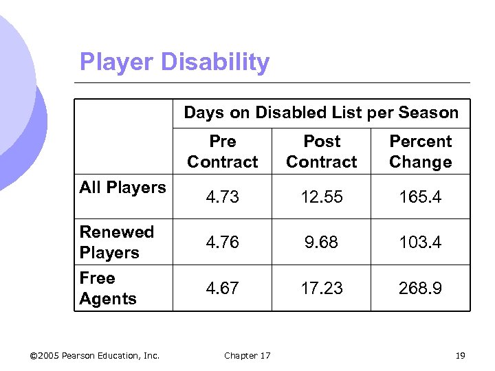Player Disability Days on Disabled List per Season Pre Contract All Players Renewed Players Free Agents © 2005 Pearson Education, Inc. Post Contract Percent Change 4. 73 12. 55 165. 4 4. 76 9. 68 103. 4 4. 67 17. 23 268. 9 Chapter 17 19

Lemons in Major League Baseball l Findings m Days on the disabled list increase for both free agents and renewed players. m Free agents have a significantly higher disability rate than renewed players. m This indicates a lemons market. © 2005 Pearson Education, Inc. Chapter 17 20

Market Signaling l The process of sellers using signals to convey information to buyers about the product’s quality. l For example, how do workers let employers know they are productive so they will be hired? © 2005 Pearson Education, Inc. Chapter 17 21

Market Signaling l Weak signal could be dressing well m Is weak because even unproductive employees can dress well l Strong Signal m To be effective, a signal must be easier for high quality sellers to give than low quality sellers. m Example l Highly productive workers signal with educational attainment level. © 2005 Pearson Education, Inc. Chapter 17 22

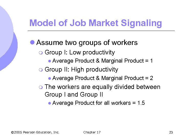Model of Job Market Signaling l Assume two groups of workers m Group I: Low productivity l Average m Group Product & Marginal Product = 1 II: High productivity l Average Product & Marginal Product = 2 m The workers are equally divided between Group I and Group II l Average © 2005 Pearson Education, Inc. Product for all workers = 1. 5 Chapter 17 23

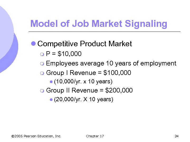Model of Job Market Signaling l Competitive Product Market m. P = $10, 000 m Employees average 10 years of employment m Group I Revenue = $100, 000 l (10, 000/yr. m Group II Revenue = $200, 000 l (20, 000/yr. © 2005 Pearson Education, Inc. x 10 years) X 10 years) Chapter 17 24

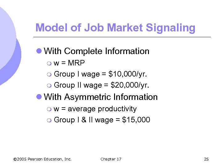Model of Job Market Signaling l With Complete Information mw = MRP m Group I wage = $10, 000/yr. m Group II wage = $20, 000/yr. l With Asymmetric Information mw = average productivity m Group I & II wage = $15, 000 © 2005 Pearson Education, Inc. Chapter 17 25

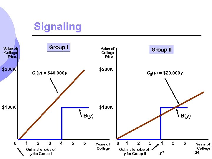
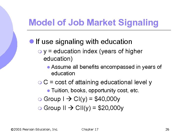Model of Job Market Signaling l If use signaling with education my = education index (years of higher education) l Assume all benefits encompassed in years of education m. C = cost of attaining educational level y l Tuition, books, opportunity cost, etc. m Group I CI(y) = $40, 000 y m Group II CII(y) = $20, 000 y © 2005 Pearson Education, Inc. Chapter 17 26

Model of Job Market Signaling l Cost of education is greater for the low productivity group than for high productivity group m Low productivity workers may simply be less studious m Low productivity workers progress more slowly through degree program © 2005 Pearson Education, Inc. Chapter 17 27

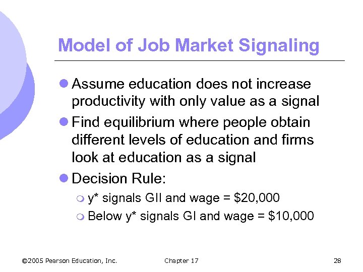Model of Job Market Signaling l Assume education does not increase productivity with only value as a signal l Find equilibrium where people obtain different levels of education and firms look at education as a signal l Decision Rule: m y* signals GII and wage = $20, 000 m Below y* signals GI and wage = $10, 000 © 2005 Pearson Education, Inc. Chapter 17 28

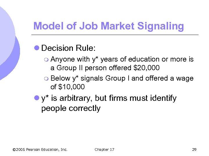Model of Job Market Signaling l Decision Rule: m Anyone with y* years of education or more is a Group II person offered $20, 000 m Below y* signals Group I and offered a wage of $10, 000 l y* is arbitrary, but firms must identify people correctly © 2005 Pearson Education, Inc. Chapter 17 29

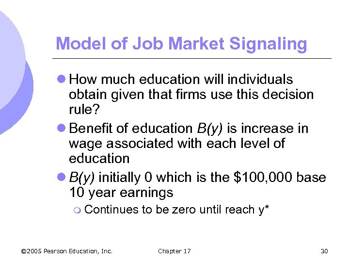Model of Job Market Signaling l How much education will individuals obtain given that firms use this decision rule? l Benefit of education B(y) is increase in wage associated with each level of education l B(y) initially 0 which is the $100, 000 base 10 year earnings m Continues © 2005 Pearson Education, Inc. to be zero until reach y* Chapter 17 30

Model of Job Market Signaling l There is no reason the obtain an education level between 0 and y* because earnings are the same l Similarly, there is no incentive to obtain more than y* level of education because once hit the y* level of pay, there are no more increases in wages © 2005 Pearson Education, Inc. Chapter 17 31

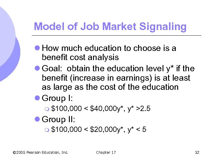Model of Job Market Signaling l How much education to choose is a benefit cost analysis l Goal: obtain the education level y* if the benefit (increase in earnings) is at least as large as the cost of the education l Group I: m $100, 000 < $40, 000 y*, y* >2. 5 l Group II: m $100, 000 © 2005 Pearson Education, Inc. < $20, 000 y*, y* < 5 Chapter 17 32

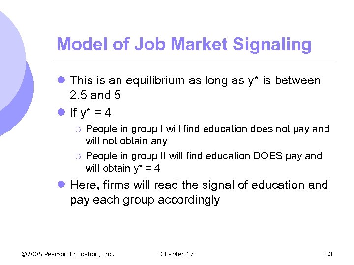Model of Job Market Signaling l This is an equilibrium as long as y* is between 2. 5 and 5 l If y* = 4 m m People in group I will find education does not pay and will not obtain any People in group II will find education DOES pay and will obtain y* = 4 l Here, firms will read the signal of education and pay each group accordingly © 2005 Pearson Education, Inc. Chapter 17 33

Signaling Group I Value of College Educ. $200 K Value of College Educ. Group II $200 K CI(y) = $40, 000 y $100 K CII(y) = $20, 000 y $100 K B(y) 0 1 2 3 4 Optimal choice of © 2005 Pearson Education, y* Inc. y for Group I 5 6 B(y) Years of College 0 1 2 3 Optimal choice of y for Group II 4 y* 5 6 Years of College 34

Signaling l Education does increase productivity and provides a useful signal about individual work habits even if education does not change productivity. © 2005 Pearson Education, Inc. Chapter 17 35

Market Signaling l Guarantees and Warranties m Signaling to identify high quality and dependability m Effective decision tool because the cost of warranties to low-quality producers is too high © 2005 Pearson Education, Inc. Chapter 17 36

Moral Hazard l Moral hazard occurs when the insured party whose actions are unobserved can affect the probability or magnitude of a payment associated with an event. m If my home is insured, I might be less likely to lock my doors or install a security system m Individual may change behavior because of insurance – moral hazard © 2005 Pearson Education, Inc. Chapter 17 37

Moral Hazard l Determining the Premium for Fire Insurance m Warehouse worth $100, 000 m Probability of a fire: l. 005 with a $50 fire prevention program l. 01 without the program m If the insurance company cannot monitor to see if he program was run, how do they determine premiums? © 2005 Pearson Education, Inc. Chapter 17 38

Moral Hazard l With the program the premium is: m. 005 x $100, 000 = $500 l Once insured owners purchase the insurance, the owners no longer have an incentive to run the program, therefore the probability of loss is. 01 l $500 premium will lead to a loss because the expected loss is now $1, 000 (. 01 x $100, 000) © 2005 Pearson Education, Inc. Chapter 17 39

Moral Hazard l Moral hazard is not only a problem for insurance companies, but it alters the ability of markets to allocate resources efficiently. l Consider the demand (MB) of driving m If there is no moral hazard, marginal cost of driving is MC m Increasing miles will increase insurance premium and the total cost of driving © 2005 Pearson Education, Inc. Chapter 17 40

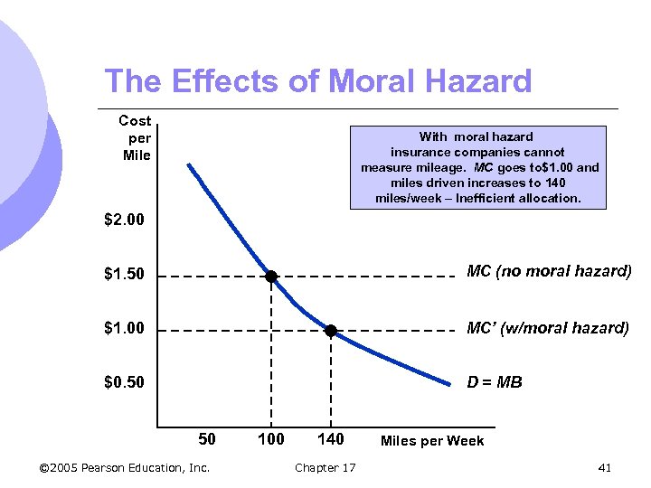The Effects of Moral Hazard Cost per Mile With moral hazard insurance companies cannot measure mileage. MC goes to$1. 00 and miles driven increases to 140 miles/week – Inefficient allocation. $2. 00 $1. 50 MC (no moral hazard) $1. 00 MC’ (w/moral hazard) $0. 50 D = MB 50 © 2005 Pearson Education, Inc. 100 140 Chapter 17 Miles per Week 41

Reducing Moral Hazard – Warranties of Animal Health l Scenario m Livestock buyers want disease free animals. m Asymmetric information exists m Many states require warranties m Buyers and sellers no longer have an incentive to reduce disease (moral hazard). © 2005 Pearson Education, Inc. Chapter 17 42

The Principal – Agent Problem l Owners cannot completely monitor their employees – employees are better informed than owners l This creates a principal-agent problem which arises when agents pursue their own goals, rather than the goals of the principal. © 2005 Pearson Education, Inc. Chapter 17 43

The Principal – Agent Problem l Company owners are principals. l Workers and managers are agents. l Owners do not have complete knowledge. l Employees may pursue their own goals even at a cost of reduce profits. © 2005 Pearson Education, Inc. Chapter 17 44

The Principal – Agent Problem l The Principal – Agent Problem in Private Enterprises m Only 16 of 100 largest corporations have individual family or financial institution ownership exceeding 10%. m Most large firms are controlled by management. m Monitoring management is costly (asymmetric information). © 2005 Pearson Education, Inc. Chapter 17 45

The Principal – Agent Problem – Private Enterprises l Managers may pursue their own objectives. m Growth and larger market share to increase cash flow and therefore perks to the manager m Utility from job from profit and from respect of peers, power to control corporation, fringe benefits, long job tenure, etc. © 2005 Pearson Education, Inc. Chapter 17 46

The Principal – Agent Problem – Private Enterprises l Limitations to managers’ ability to deviate from objective of owners m Stockholders can oust managers m Takeover attempts if firm is poorly managed m Market for managers who maximize profits – those that perform get paid more so incentive to act for the firm © 2005 Pearson Education, Inc. Chapter 17 47

The Principal – Agent Problem – Private Enterprises l The problem of limited stockholder control shows up in executive compensation m Business Week showed that average CEO earned $13. 1 million and has continued to increase at a double-digit rate m For 10 public companies led by highest paid CEOs, there was negative correlation between CEO pay and company performance © 2005 Pearson Education, Inc. Chapter 17 48

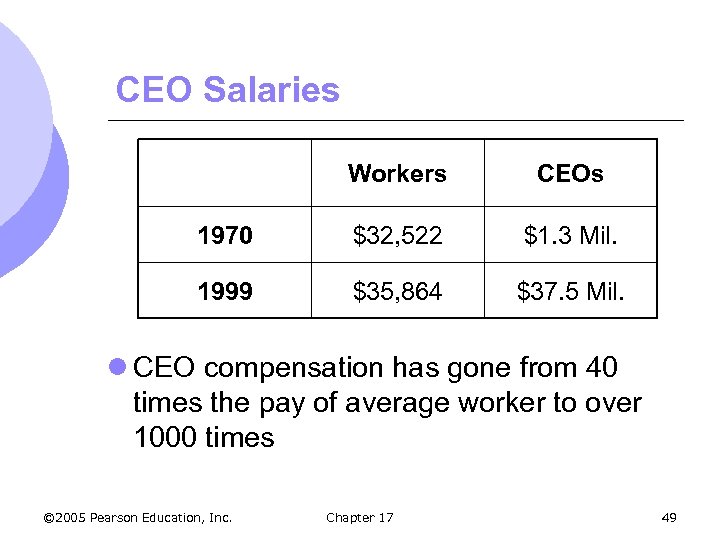CEO Salaries Workers CEOs 1970 $32, 522 $1. 3 Mil. 1999 $35, 864 $37. 5 Mil. l CEO compensation has gone from 40 times the pay of average worker to over 1000 times © 2005 Pearson Education, Inc. Chapter 17 49

CEO Salaries l Although originally thought that executive compensation reflected reward for talent, recent evidence suggests managers have been able to manipulate boards to extract compensation out of line with economic contribution © 2005 Pearson Education, Inc. Chapter 17 50

CEO Salaries l How have they been able to do this? 1. 2. Boards don’t typically have necessary information and independence to negotiate effectively Managers have introduced forms of compensation that camouflage the extraction of rents from shareholders m Stock options (not counted as expenses) © 2005 Pearson Education, Inc. Chapter 17 51

CEO Salaries l Rent extraction has increased as consultants are hired to determine appropriate pay for CEO l Firm usually wants to provide at least the average of other companies, so salaries have been rising rapidly l With publicity increasing, CEO salaries seem to be rising less rapidly © 2005 Pearson Education, Inc. Chapter 17 52

The Principal – Agent Problem – Public Enterprises l Observations m Managers’ goals may deviate from the agencies goal (size) m Oversight is difficult (asymmetric information) m Market forces are lacking © 2005 Pearson Education, Inc. Chapter 17 53

The Principal – Agent Problem l Limitations to Management Power m Managers choose a public service position m Managerial job market m Legislative and agency oversight (GAO & OMB) m Competition among agencies © 2005 Pearson Education, Inc. Chapter 17 54

The Managers of Nonprofit Hospitals as Agents l Are non-profit organizations more or less efficient that for-profit firms? m 725 hospitals from 14 hospital chains m Return on investment (ROI) and average cost (AC) measured © 2005 Pearson Education, Inc. Chapter 17 55

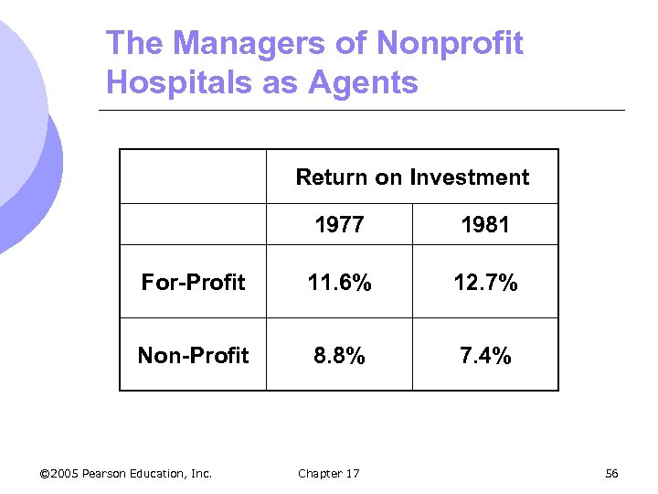The Managers of Nonprofit Hospitals as Agents Return on Investment 1977 1981 For-Profit 11. 6% 12. 7% Non-Profit 8. 8% 7. 4% © 2005 Pearson Education, Inc. Chapter 17 56

The Managers of Nonprofit Hospitals as Agents l After adjusting for differences in services: m AC/patient day in nonprofits is 8% greater than profits m Conclusion l Profit incentive impacts performance m Cost and benefits of subsidizing nonprofits must be considered. © 2005 Pearson Education, Inc. Chapter 17 57

Incentives in the Principal-Agent Framework l Designing a reward system to align the principal and agent’s goals--an example m Watch manufacturer m Uses labor and machinery m Owners goal is to maximize profit m Machine repairperson can influence reliability of machines and profits © 2005 Pearson Education, Inc. Chapter 17 58

Incentives in the Principal-Agent Framework l Designing a reward system to align the principal and agent’s goals--an example m Revenue also depends, in part, on the quality of parts and the reliability of labor. m High monitoring cost makes it difficult to assess the repair-person’s work © 2005 Pearson Education, Inc. Chapter 17 59

Incentives in the Principal-Agent Framework l Small manufacturer uses labor and machinery to produce watches l Goal to maximize profits l High monitoring costs keep owners from measuring the effort of the repairperson directly © 2005 Pearson Education, Inc. Chapter 17 60

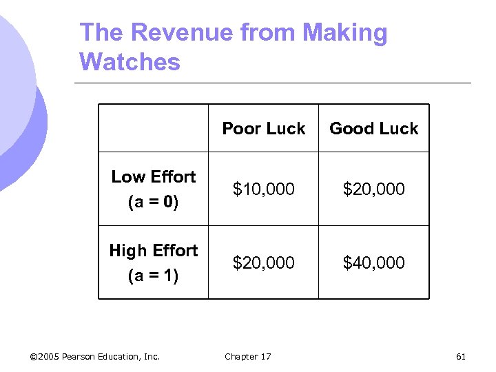The Revenue from Making Watches Poor Luck Good Luck Low Effort (a = 0) $10, 000 $20, 000 High Effort (a = 1) $20, 000 $40, 000 © 2005 Pearson Education, Inc. Chapter 17 61

Incentives in the Principal-Agent Framework l Designing a reward system to align the principal and agent’s goals--an example m Repairperson can work with either high or low effort m Revenues depend on effort relative to the other events (poor or good luck) m Owners cannot determine a high or low effort when revenue = $20, 000 © 2005 Pearson Education, Inc. Chapter 17 62

Incentives in the Principal-Agent Framework l Designing a reward system to align the principal and agent’s goals--an example m Repairperson’s goal is to maximize wage net of cost m Cost = 0 for low effort m Cost = $10, 000 for high effort m w(R) = repairperson wage based only on output © 2005 Pearson Education, Inc. Chapter 17 63

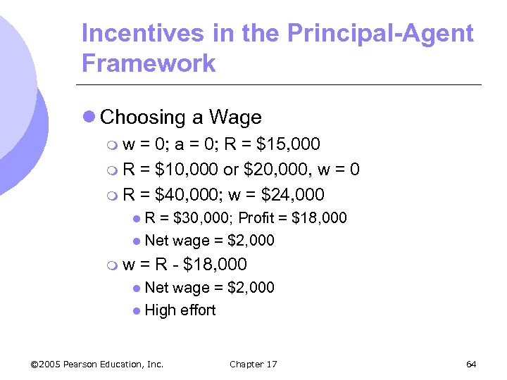Incentives in the Principal-Agent Framework l Choosing a Wage mw = 0; a = 0; R = $15, 000 m R = $10, 000 or $20, 000, w = 0 m R = $40, 000; w = $24, 000 l. R = $30, 000; Profit = $18, 000 l Net wage = $2, 000 mw = R - $18, 000 l Net wage = $2, 000 l High effort © 2005 Pearson Education, Inc. Chapter 17 64

Incentives in the Principal-Agent Framework l Conclusion m Incentive structure that rewards the outcome of high levels of effort can induce agents to aim for the goals set by the principals. © 2005 Pearson Education, Inc. Chapter 17 65

Managerial Incentives in an Integrated Firm l In integrated firms, division managers have better (asymmetric) information about production than central management l Two Issues m How can central management illicit accurate information m How can central management achieve efficient divisional production © 2005 Pearson Education, Inc. Chapter 17 66

Managerial Incentives in an Integrated Firm l We will focus on firms that are integrated l Horizontally integrated m Several plants produce the same or related products l Vertically integrated m Form contains several divisions, with some producing parts and components that others use to produce finished products © 2005 Pearson Education, Inc. Chapter 17 67

Managerial Incentives in an Integrated Firm l Possible Incentive Plans 1. Give plant managers bonuses based on either total output or operating profit m m m Would encourage mangers to maximize output Would penalize managers whose plants have higher costs and lower capacity No incentive to obtain and reveal accurate cost and capacity information © 2005 Pearson Education, Inc. Chapter 17 68

Managerial Incentives in an Integrated Firm 2. Ask managers about their costs and capacities and then base bonuses on how well they do relative to their answers Qf = estimate of feasible production level l B = bonus in dollars l Q = actual output l B = 10, 000 -. 5(Qf - Q) l m Incentive to underestimate Qf © 2005 Pearson Education, Inc. Chapter 17 69

Managerial Incentives in an Integrated Firm l If manager estimates capacity to be 18, 000 rather than 20, 000. If the plant only produces 16, 000 her bonus increases from $8000 to $9000 m Don’t get accurate information about capacity and don’t insure efficiency l Bonus still tied to accuracy of forecast © 2005 Pearson Education, Inc. Chapter 17 70

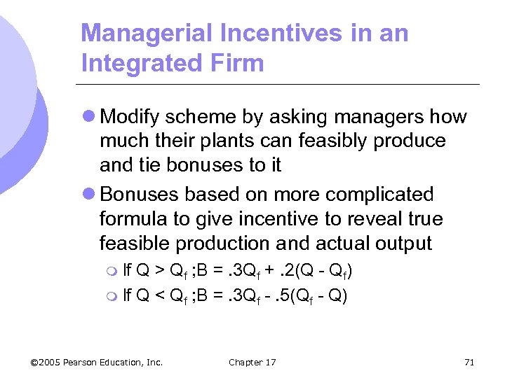Managerial Incentives in an Integrated Firm l Modify scheme by asking managers how much their plants can feasibly produce and tie bonuses to it l Bonuses based on more complicated formula to give incentive to reveal true feasible production and actual output m If Q > Qf ; B =. 3 Qf +. 2(Q - Qf) m If Q < Qf ; B =. 3 Qf -. 5(Qf - Q) © 2005 Pearson Education, Inc. Chapter 17 71

Managerial Incentives in an Integrated Firm l Assume true production limit is Q* = 20, 000 m Line for 20, 000 is continued for outputs beyond 20, 000 to illustrate the bonus scheme but dashed to dignify the infeasibility of such production m Bonus is maximized when firm produces at its limit of 20, 000; the bonus is then $6000 © 2005 Pearson Education, Inc. Chapter 17 72

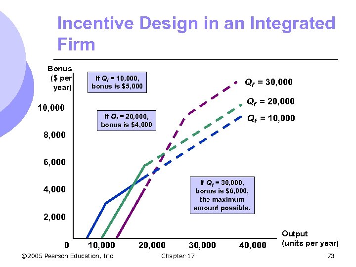Incentive Design in an Integrated Firm Bonus ($ per year) 10, 000 If Qf = 10, 000, bonus is $5, 000 Qf = 30, 000 Qf = 20, 000 If Qf = 20, 000, bonus is $4, 000 Qf = 10, 000 8, 000 6, 000 If Qf = 30, 000, bonus is $6, 000, the maximum amount possible. 4, 000 2, 000 0 10, 000 © 2005 Pearson Education, Inc. 20, 000 30, 000 Chapter 17 40, 000 Output (units per year) 73

Efficiency Wage Theory l In a competitive labor market, all who wish to work will find jobs for a wage equal to their marginal product. m However, most countries’ economies experience unemployment. © 2005 Pearson Education, Inc. Chapter 17 74

Efficiency Wage Theory l The efficiency wage theory can explain the presence of unemployment and wage discrimination. m In developing countries, productivity depends on the wage rate for nutritional reasons. © 2005 Pearson Education, Inc. Chapter 17 75

Efficiency Wage Theory l The shirking model can be better used to explain unemployment and wage discrimination in the United States. m Assumes perfectly competitive markets m However, workers can work or shirk. m Since performance information is limited, workers may not get fired. © 2005 Pearson Education, Inc. Chapter 17 76

Efficiency Wage Theory l If workers paid market clearing wage w*, they have incentive to shirk l If get caught and fired, they can immediately get a job elsewhere for same wage l Firms have to pay a higher wage to make loss higher from shirking l Wage at which no shirking occurs is the efficiency wage © 2005 Pearson Education, Inc. Chapter 17 77

Efficiency Wage Theory l All firms will offer more than market clearing wage, w*, say we (efficiency wage) l In this case workers fired for shirking face unemployment because demand for labor is less than market clearing quantity © 2005 Pearson Education, Inc. Chapter 17 78

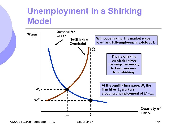Unemployment in a Shirking Model Wage Demand for Labor No-Shirking Constraint Without shirking, the market wage is w*, and full-employment exists at L* SL The no-shirking constraint gives the wage necessary to keep workers from shirking. At the equilibrium wage, We the firm hires Le workers creating unemployment of L* - Le. we w* Le © 2005 Pearson Education, Inc. L* Chapter 17 Quantity of Labor 79

Efficiency Wages at Ford Motor Company l Labor turnover at Ford m 1913: 380% m 1914: 1000% l Average pay = $2 - $3 l Ford increased pay to $5 © 2005 Pearson Education, Inc. Chapter 17 80

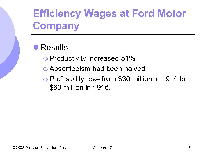Efficiency Wages at Ford Motor Company l Results m Productivity increased 51% m Absenteeism had been halved m Profitability rose from $30 million in 1914 to $60 million in 1916. © 2005 Pearson Education, Inc. Chapter 17 81