Chapter 17 Choice Making Under Uncertainty 17 1

Chapter 17 Choice Making Under Uncertainty 17/1 © 2009 Pearson Education Canada

Calculating Expected Monetary Value u The expected monetary value is simply the weighted average of the payoffs (the possible outcomes), where the weights are the probabilities of occurrence assigned to each outcome. 17/2 © 2009 Pearson Education Canada

Expected Value u Given: Two possible outcomes having payoffs X 1 and X 2 and probabilities of each outcome given by Pr 1 & Pr 2. u The expected value (EV) can be expressed as: EV(X) = Pr 1 X 1+ Pr 2 X 2 17/3 © 2009 Pearson Education Canada

Expected Utility Hypothesis u Expected utility is calculated the same way as expected monetary value, except that the utility associated with a payoff is substituted for its monetary value. u With two outcomes for wealth ($200 and $0) and with each outcome occurring ½ the time, the expected utility can be written: E(u) = (1/2)U($200) + (1/2)U($0) 17/4 © 2009 Pearson Education Canada

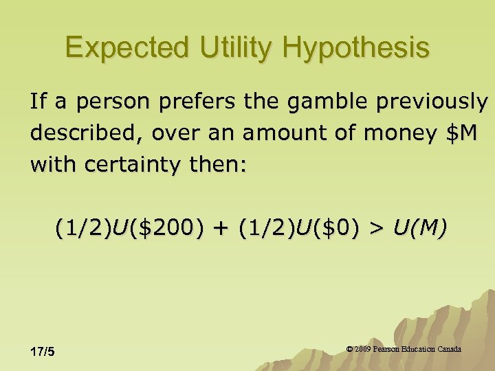Expected Utility Hypothesis If a person prefers the gamble previously described, over an amount of money $M with certainty then: (1/2)U($200) + (1/2)U($0) > U(M) 17/5 © 2009 Pearson Education Canada

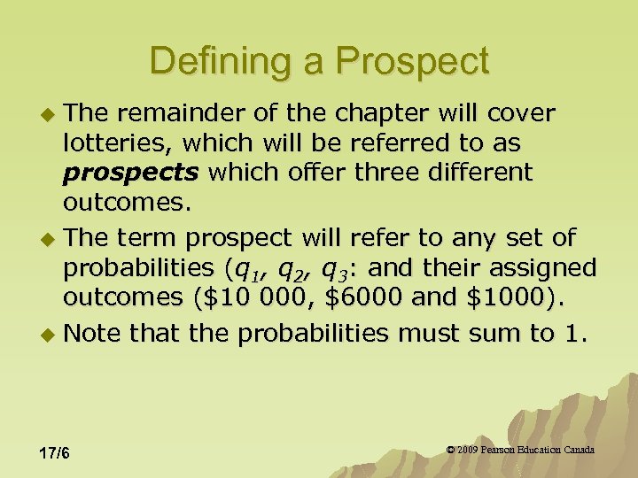Defining a Prospect The remainder of the chapter will cover lotteries, which will be referred to as prospects which offer three different outcomes. u The term prospect will refer to any set of probabilities (q 1, q 2, q 3: and their assigned outcomes ($10 000, $6000 and $1000). u Note that the probabilities must sum to 1. u 17/6 © 2009 Pearson Education Canada

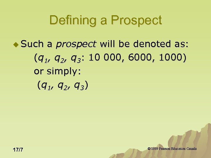Defining a Prospect u Such a prospect will be denoted as: (q 1, q 2, q 3: 10 000, 6000, 1000) or simply: ( q 1 , q 2 , q 3 ) 17/7 © 2009 Pearson Education Canada

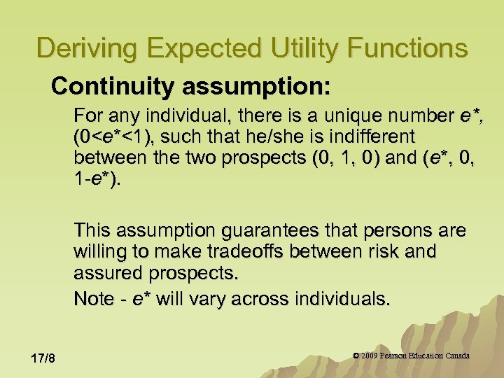Deriving Expected Utility Functions Continuity assumption: For any individual, there is a unique number e*, (0

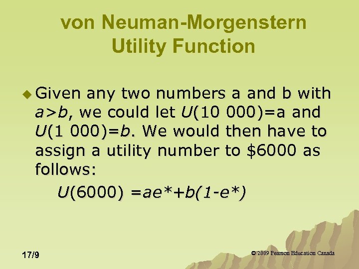von Neuman-Morgenstern Utility Function u Given any two numbers a and b with a>b, we could let U(10 000)=a and U(1 000)=b. We would then have to assign a utility number to $6000 as follows: U(6000) =ae*+b(1 -e*) 17/9 © 2009 Pearson Education Canada

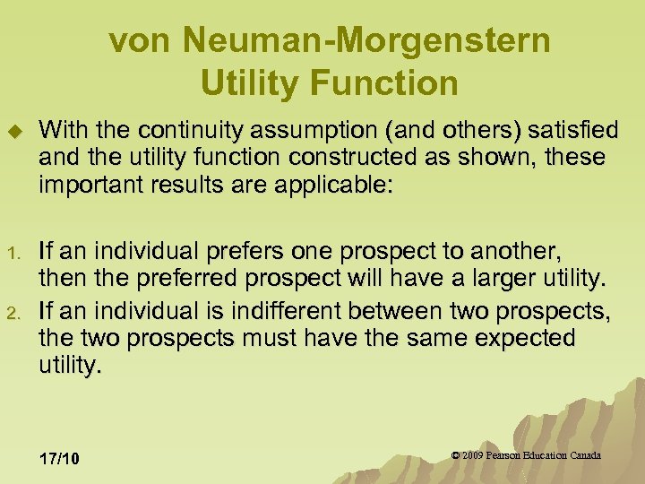von Neuman-Morgenstern Utility Function u With the continuity assumption (and others) satisfied and the utility function constructed as shown, these important results are applicable: 1. If an individual prefers one prospect to another, then the preferred prospect will have a larger utility. If an individual is indifferent between two prospects, the two prospects must have the same expected utility. 2. 17/10 © 2009 Pearson Education Canada

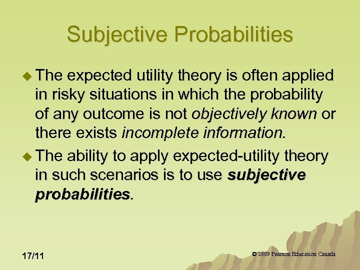Subjective Probabilities u The expected utility theory is often applied in risky situations in which the probability of any outcome is not objectively known or there exists incomplete information. u The ability to apply expected-utility theory in such scenarios is to use subjective probabilities. 17/11 © 2009 Pearson Education Canada

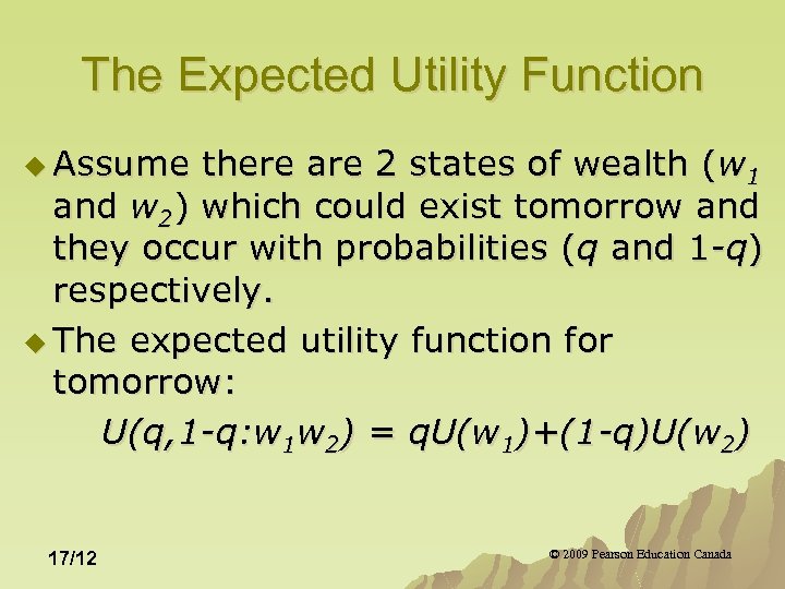The Expected Utility Function u Assume there are 2 states of wealth (w 1 and w 2) which could exist tomorrow and they occur with probabilities (q and 1 -q) respectively. u The expected utility function for tomorrow: U(q, 1 -q: w 1 w 2) = q. U(w 1)+(1 -q)U(w 2) 17/12 © 2009 Pearson Education Canada

The Expected Utility Function u 1. 2. Two key features of this utility functions: The U functions are cardinal, meaning that the utility values have specific meaning in relation to one another. This expected utility function is linear in its probabilities (which simplifies MRS). 17/13 © 2009 Pearson Education Canada

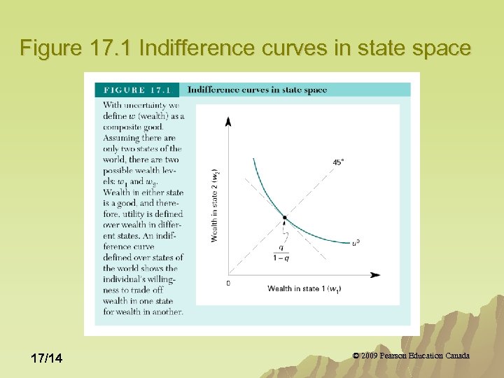Figure 17. 1 Indifference curves in state space 17/14 © 2009 Pearson Education Canada

From Figure 17. 1 shows an indifference curve for utility level u. Wealth in state 1(today) and state 2 (tomorrow) are on each axis. u q and (1 -q) are fixed. u The MRS (slope of u 0) shows the rate at which an individual trades wealth in state 1 for wealth in state 2, before either of these states occur. u 17/15 © 2009 Pearson Education Canada

From Figure 17. 1 The slope of the indifference curve is equal to the ratio of the probabilities times the ratio of the marginal utilities. u Each marginal utility, however, is function of wealth in only one state, since the utility functions are the same in each state. u Therefore, the MRS equals the ratio of the probabilities. u 17/16 © 2009 Pearson Education Canada

From Figure 17. 1 Hence, along the 45 degree line, where wealth in the two states are equal, the slope of u 0 is q/(1 -q). u If q is large relative to (1 -q) then u 0 is relatively steep and vice versa. u In other words, if you believe state 1 is very likely (q is high) then you will prefer your wealth in state one rather than state two. u 17/17 © 2009 Pearson Education Canada

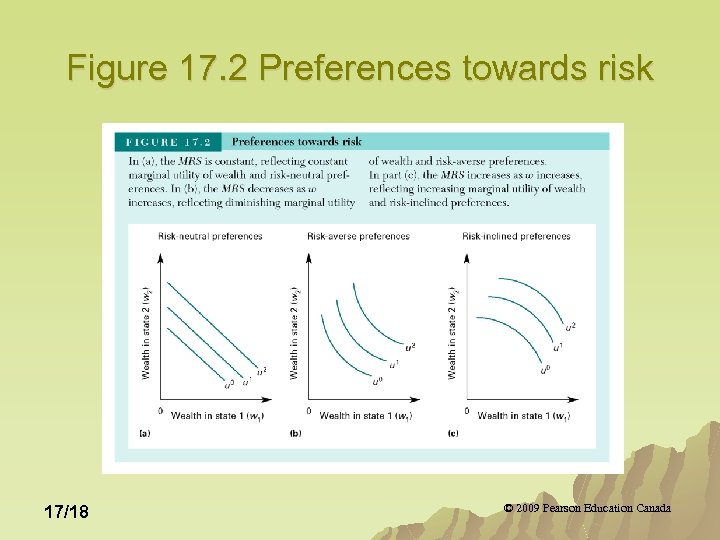Figure 17. 2 Preferences towards risk 17/18 © 2009 Pearson Education Canada

Optimal Risk Bearing Now that different attitudes toward risk have been defined, it is necessary to illustrate how attitudes toward risk affect choices over risky prospects. u An expected value line shows prospects with the same expected value. Note however that along this line, the risk of each prospect varies. u 17/19 © 2009 Pearson Education Canada

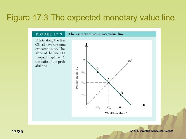Figure 17. 3 The expected monetary value line 17/20 © 2009 Pearson Education Canada

From Figure 17. 3 At point A there is no risk and that risk increases as the prospects move away from the 45 degree line. u The slope of the expected value line equals the ratios of the probabilities (relative prices) u Utility will be maximized when the individual’s MRS equals the ratios of the probabilities. u 17/21 © 2009 Pearson Education Canada

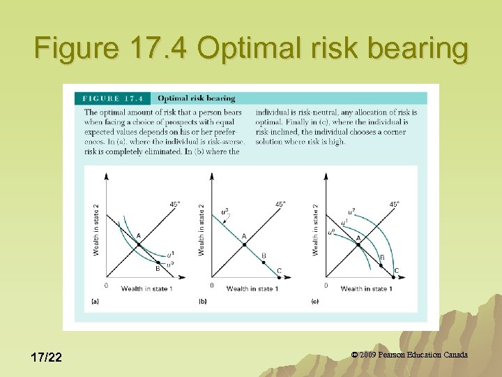Figure 17. 4 Optimal risk bearing 17/22 © 2009 Pearson Education Canada

Optimal Risk Bearing The optimal amount of risk that a person bears in life depends on his/her aversion to risk. u The choices of risk averse persons tend toward the 45 degree line where wealth is the same no matter what state arises. u Risk inclined persons move away from the 45 degree line and are willing to take the chance that they will be better off in one state compared to the other. u 17/23 © 2009 Pearson Education Canada

Pooling Risk Pooling is a form of insurance aimed at reducing an individual’s exposure to risk by spreading that risk over a larger number of persons. u Suppose the probability of either Abe or Martha having a fire is 1 -q, the loss from such a fire is L dollars and wealth in period t denoted as wt. u 17/24 © 2009 Pearson Education Canada

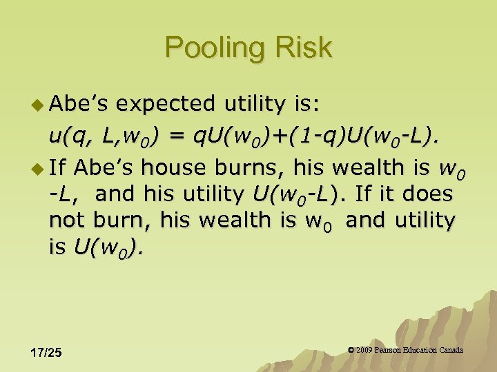Pooling Risk u Abe’s expected utility is: u(q, L, w 0) = q. U(w 0)+(1 -q)U(w 0 -L). u If Abe’s house burns, his wealth is w 0 -L, and his utility U(w 0 -L). If it does not burn, his wealth is w 0 and utility is U(w 0). 17/25 © 2009 Pearson Education Canada

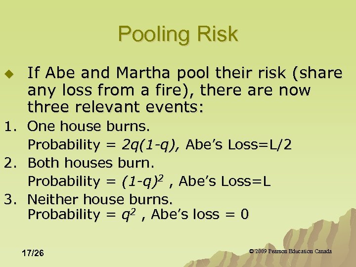Pooling Risk u If Abe and Martha pool their risk (share any loss from a fire), there are now three relevant events: 1. One house burns. Probability = 2 q(1 -q), Abe’s Loss=L/2 2. Both houses burn. Probability = (1 -q)2 , Abe’s Loss=L 3. Neither house burns. Probability = q 2 , Abe’s loss = 0 17/26 © 2009 Pearson Education Canada

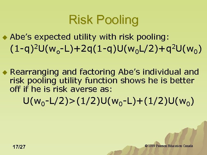Risk Pooling u Abe’s expected utility with risk pooling: (1 -q)2 U(wo-L)+2 q(1 -q)U(w 0 L/2)+q 2 U(w 0) u Rearranging and factoring Abe’s individual and risk pooling utility function shows he is better off if he is risk averse as: U(w 0 -L/2)>(1/2)U(w 0 -L)+(1/2)U(w 0) 17/27 © 2009 Pearson Education Canada

Risk Pooling u When individuals are risk averse, they have clear incentives to create institutions that allow them to share (pool) their risks. 17/28 © 2009 Pearson Education Canada

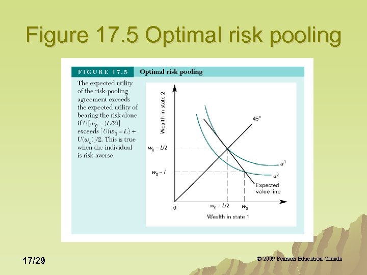Figure 17. 5 Optimal risk pooling 17/29 © 2009 Pearson Education Canada

The Market for Insurance u What is Abe’s reservation demand price for insurance (the maximum he is willing to pay rather than go without)? u Set his expected utility without insurance equal to the certainty equivalent (assured prospect wce in Figure 17. 6). 17/30 © 2009 Pearson Education Canada

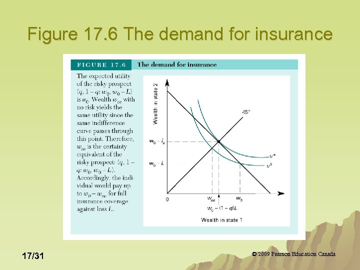Figure 17. 6 The demand for insurance 17/31 © 2009 Pearson Education Canada

The Market for Insurance u On the assumption that insurance companies are risk neutral, what is the lowest price they will offer full coverage? u This is the reservation supply price, denoted by Is in Figure 17. 6 17/32 © 2009 Pearson Education Canada

The Market for Insurance u Ignoring any administrative costs, the expected costs are (1 -q)L and the firm will write a policy if revenues (I) exceed costs. 17/33 © 2009 Pearson Education Canada

The Market for Insurance As shown in Figure 17. 6, there is a viable insurance market because the reservation supply price Is =(1 -q)L is less than the reservation demand price (distance w 0 -wce). u Abe trades his risky prospect for the assured prospect and reaches indifference curve u*. u If no resources are required to write and administer insurance policies and if individuals are risk-averse, there is a viable market for insurance. u 17/34 © 2009 Pearson Education Canada