8c8c21f2c420262ed164cba2ebbd0b08.ppt
- Количество слайдов: 32
 Chapter 17 Choice Making Under Uncertainty 17. 1 © 2005 Pearson Education Canada Inc.
 Calculating Expected Monetary Value u The expected monetary value is simply the weighted average of the payoffs (the possible outcomes), where the weights are the probabilities of occurrence assigned to each outcome. 17. 2 © 2005 Pearson Education Canada Inc.
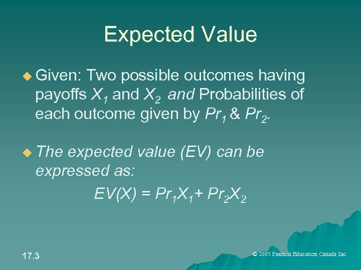 Expected Value u Given: Two possible outcomes having payoffs X 1 and X 2 and Probabilities of each outcome given by Pr 1 & Pr 2. u The expected value (EV) can be expressed as: EV(X) = Pr 1 X 1+ Pr 2 X 2 17. 3 © 2005 Pearson Education Canada Inc.
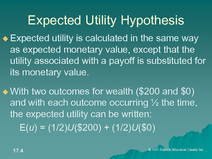 Expected Utility Hypothesis u Expected utility is calculated in the same way as expected monetary value, except that the utility associated with a payoff is substituted for its monetary value. u With two outcomes for wealth ($200 and $0) and with each outcome occurring ½ the time, the expected utility can be written: E(u) = (1/2)U($200) + (1/2)U($0) 17. 4 © 2005 Pearson Education Canada Inc.
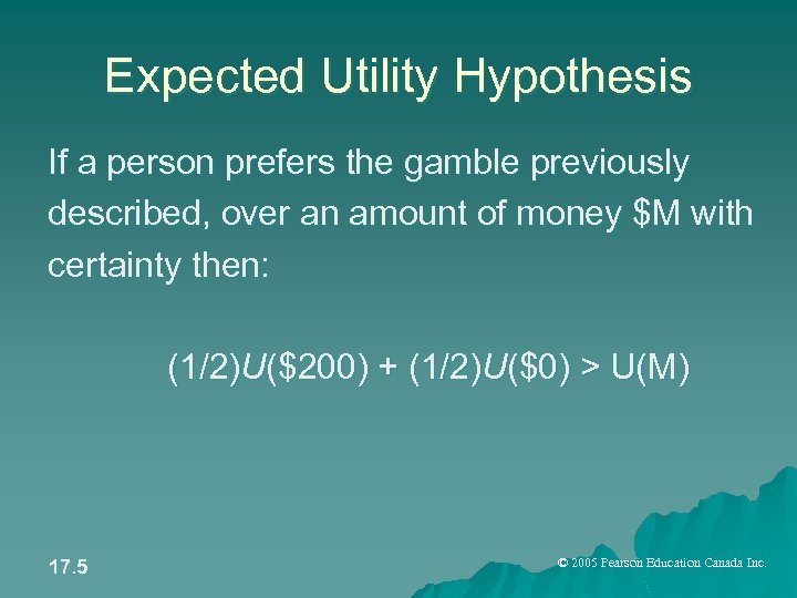 Expected Utility Hypothesis If a person prefers the gamble previously described, over an amount of money $M with certainty then: (1/2)U($200) + (1/2)U($0) > U(M) 17. 5 © 2005 Pearson Education Canada Inc.
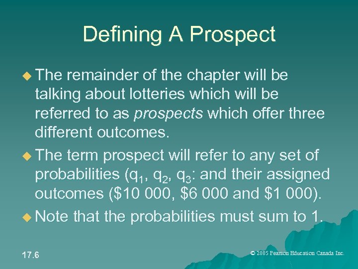 Defining A Prospect u The remainder of the chapter will be talking about lotteries which will be referred to as prospects which offer three different outcomes. u The term prospect will refer to any set of probabilities (q 1, q 2, q 3: and their assigned outcomes ($10 000, $6 000 and $1 000). u Note that the probabilities must sum to 1. 17. 6 © 2005 Pearson Education Canada Inc.
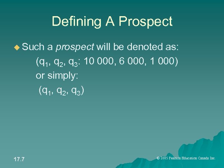 Defining A Prospect u Such a prospect will be denoted as: (q 1, q 2, q 3: 10 000, 6 000, 1 000) or simply: (q 1, q 2, q 3) 17. 7 © 2005 Pearson Education Canada Inc.
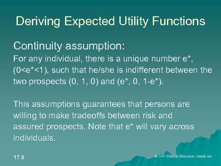 Deriving Expected Utility Functions Continuity assumption: For any individual, there is a unique number e*, (0
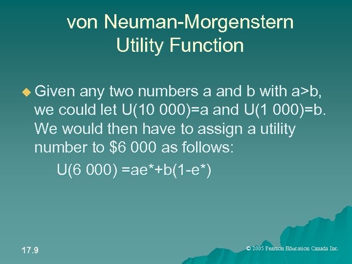 von Neuman-Morgenstern Utility Function u Given any two numbers a and b with a>b, we could let U(10 000)=a and U(1 000)=b. We would then have to assign a utility number to $6 000 as follows: U(6 000) =ae*+b(1 -e*) 17. 9 © 2005 Pearson Education Canada Inc.
 von Neuman-Morgenstern Utility Function u With the continuity assumption (and others) satisfied and the utility function constructed as shown, these important results are applicable: 1. If an individual prefers one prospect to another, then the preferred prospect will have a larger utility. If an individual is indifferent between two prospects, the two prospects must have the same expected utility. 2. 17. 10 © 2005 Pearson Education Canada Inc.
 Subjective Probabilities u The expected utility theory is often applied in risky situations in which the probability of any outcome is not objectively known or there exists incomplete information. u The ability to apply expected-utility theory is such scenarios is to use subjective probabilities. 17. 11 © 2005 Pearson Education Canada Inc.
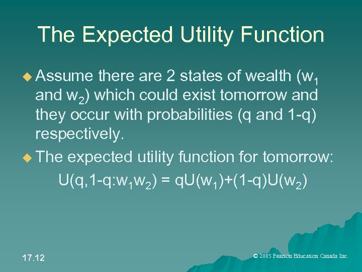 The Expected Utility Function u Assume there are 2 states of wealth (w 1 and w 2) which could exist tomorrow and they occur with probabilities (q and 1 -q) respectively. u The expected utility function for tomorrow: U(q, 1 -q: w 1 w 2) = q. U(w 1)+(1 -q)U(w 2) 17. 12 © 2005 Pearson Education Canada Inc.
 The Expected Utility Function u 1. 2. 17. 13 Two key features of this utility functions: The U functions are cardinal, meaning that the utility values have specific meaning in relation to one another. This expected utility function is linear in its probabilities (which simplifies MRS). © 2005 Pearson Education Canada Inc.
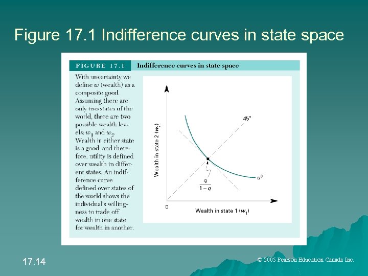 Figure 17. 1 Indifference curves in state space 17. 14 © 2005 Pearson Education Canada Inc.
 From Figure 17. 1 u Figure 17. 1 shows an indifference curve for utility level u. Wealth in state 1(today) and state 2 (tomorrow) are on each axis. u q and (1 -q) are fixed. u The MRS (slope of u 0) shows the rate at which an individual trades wealth in state 1 for wealth in state 2, before either of these states occur. 17. 15 © 2005 Pearson Education Canada Inc.
 From Figure 17. 1 u The slope of the indifference curve is equal to the ratio of the probabilities times the ratio of the marginal utilities. u Each marginal utility however is function of wealth in only one state since the utility functions are the same in each state. u Therefore the MRS equals the ratio of the probabilities. 17. 16 © 2005 Pearson Education Canada Inc.
 From Figure 17. 1 u Hence, along the 45 degree line, where wealth in the two states are equal, the slope of u 0 is q/(1 -q). u If q is large relative to (1 -q) then u 0 is relatively steep and vice versa. u In other words, if you believe state 1 is very likely (q is high) then you will prefer your wealth in state one rather than state two. 17 © 2005 Pearson Education Canada Inc.
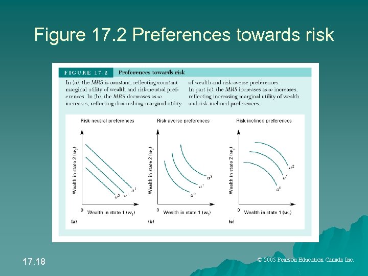 Figure 17. 2 Preferences towards risk 17. 18 © 2005 Pearson Education Canada Inc.
 Optimal Risk Bearing u Now that different attitudes toward risk have been defined, it is necessary to illustrate how attitudes toward risk affect choices over risky prospects. u An expected value line shows prospects with the same expected value. Note however that along this line, the risk of each prospect varies. 17. 19 © 2005 Pearson Education Canada Inc.
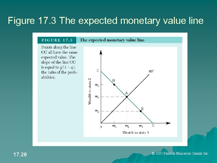 Figure 17. 3 The expected monetary value line 17. 20 © 2005 Pearson Education Canada Inc.
 From Figure 17. 3 u At point A there is no risk and that risk increases as the prospects move away from the 45 degree line. u The slope of the expected value line equals the ratios of the probabilities (relative prices) u Utility will be maximized when the individual’s MRS equals the ratios of the probabilities. 17. 21 © 2005 Pearson Education Canada Inc.
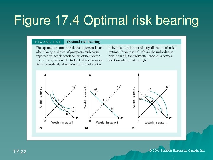 Figure 17. 4 Optimal risk bearing 17. 22 © 2005 Pearson Education Canada Inc.
 Optimal Risk Bearing u The optimal amount of risk that a person bears in life depends on his/her aversion to risk. u The choices of risk averse persons tend toward the 45 degree line where wealth is the same no matter what state arises. u Risk inclined persons move away from the 45 degree line and are willing to take the chance that they will be better off in one state compared to the other. 17. 23 © 2005 Pearson Education Canada Inc.
 Pooling Risk u Risk Pooling is a form of insurance aimed at reducing an individual’s exposure to risk by spreading that risk over a larger number of persons. u Suppose the probability of either Abe or Martha having a fire is 1 -q, the loss from such a fire is L dollars and wealth in period t denoted as wt. 17. 24 © 2005 Pearson Education Canada Inc.
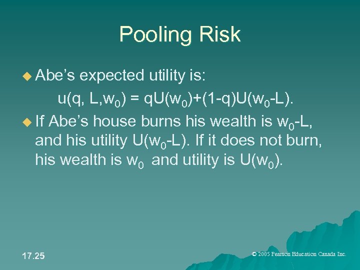 Pooling Risk u Abe’s expected utility is: u(q, L, w 0) = q. U(w 0)+(1 -q)U(w 0 -L). u If Abe’s house burns his wealth is w 0 -L, and his utility U(w 0 -L). If it does not burn, his wealth is w 0 and utility is U(w 0). 17. 25 © 2005 Pearson Education Canada Inc.
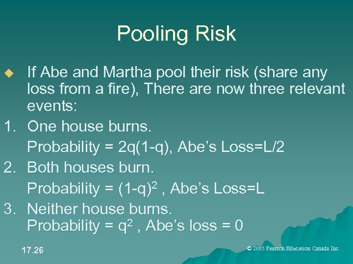 Pooling Risk If Abe and Martha pool their risk (share any loss from a fire), There are now three relevant events: 1. One house burns. Probability = 2 q(1 -q), Abe’s Loss=L/2 2. Both houses burn. Probability = (1 -q)2 , Abe’s Loss=L 3. Neither house burns. Probability = q 2 , Abe’s loss = 0 u 17. 26 © 2005 Pearson Education Canada Inc.
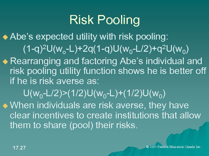 Risk Pooling u Abe’s expected utility with risk pooling: (1 -q)2 U(wo-L)+2 q(1 -q)U(w 0 -L/2)+q 2 U(w 0) u Rearranging and factoring Abe’s individual and risk pooling utility function shows he is better off if he is risk averse as: U(w 0 -L/2)>(1/2)U(w 0 -L)+(1/2)U(w 0) u When individuals are risk averse, they have clear incentives to create institutions that allow them to share (pool) their risks. 17. 27 © 2005 Pearson Education Canada Inc.
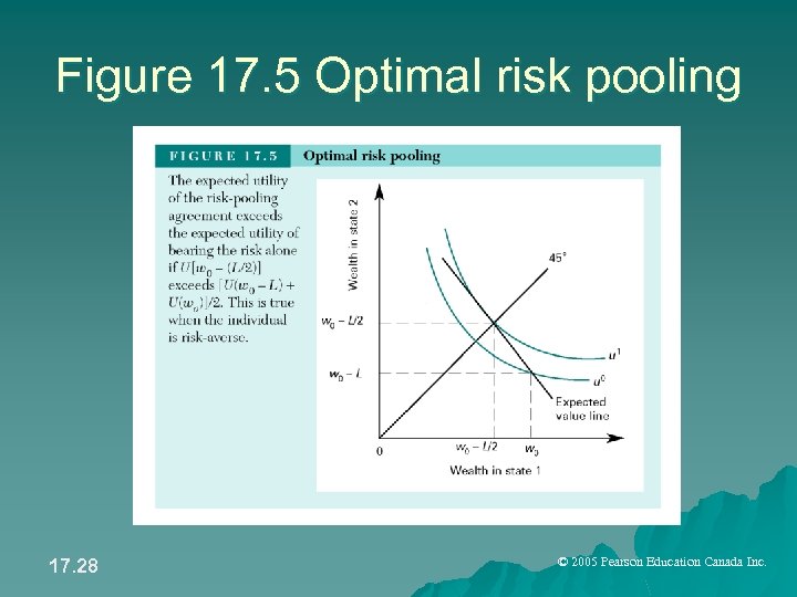 Figure 17. 5 Optimal risk pooling 17. 28 © 2005 Pearson Education Canada Inc.
 The Market for Insurance u What is Abe’s reservation demand price for insurance (the maximum he is willing to pay rather than go without)? u Set his expected utility without insurance equal to the certainty equivalent (assured prospect wce) in Figure 17. 6. 17. 29 © 2005 Pearson Education Canada Inc.
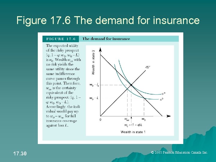 Figure 17. 6 The demand for insurance 17. 30 © 2005 Pearson Education Canada Inc.
 The Market for Insurance u On the assumption that insurance companies are risk neutral, what is the lowest price they will offer full coverage? u This is the reservation supply price, denoted by Is in Figure 17. 6 u Ignoring any administrative costs, the expected costs are (1 -q)L and the firm will write a policy if revenues (I) exceed costs. 17. 31 © 2005 Pearson Education Canada Inc.
 The Market for Insurance As shown in Figure 17. 6, there is a viable insurance market because the reservation supply price Is =(1 -q)L is less than the reservation demand price (distance w 0 wce). u Abe trades his risky prospect for the assured prospect and reaches indifference curve u*. u If no resources are required to write and administer insurance policies and if individuals are risk-averse, there is a viable market for insurance. u 17. 32 © 2005 Pearson Education Canada Inc.


