823b643dbb943e5cdc8d546212ce4242.ppt
- Количество слайдов: 48
 Chapter 16 Statistical Tests Copyright © 2014, 2011 Pearson Education, Inc. 1
 16. 1 Concepts of Statistical Tests A manager is evaluating software to filter SPAM e-mails (cost $15, 000). To make it profitable, the software must reduce SPAM to less than 20%. Should the manager buy the software? § § Use a statistical test to answer this question Consider the plausibility of a specific claim (claims are called hypotheses) Copyright © 2014, 2011 Pearson Education, Inc. 2
 16. 1 Concepts of Statistical Tests Null and Alternative Hypotheses § Statistical hypothesis: claim about a parameter of a population. § Null hypothesis (H 0): specifies a default course of action, preserves the status quo. § Alternative hypothesis (Ha): contradicts the assertion of the null hypothesis. Copyright © 2014, 2011 Pearson Education, Inc. 3
 16. 1 Concepts of Statistical Tests SPAM Software Example Let p = email that slips past the filter H 0: p ≥ 0. 20 Ha: p < 0. 20 These hypotheses lead to a one-sided test. Copyright © 2014, 2011 Pearson Education, Inc. 4
 16. 1 Concepts of Statistical Tests One- and Two-Sided Tests § One-sided test: the null hypothesis allows any value of a parameter larger (or smaller) than a specified value. § Two-sided test: the null hypothesis asserts a specific value for the population parameter. Copyright © 2014, 2011 Pearson Education, Inc. 5
 16. 1 Concepts of Statistical Tests Type I and II Errors § Reject H 0 incorrectly (buying software that will not be cost effective) § Retain H 0 incorrectly (not buying software that would have been cost effective) Copyright © 2014, 2011 Pearson Education, Inc. 6
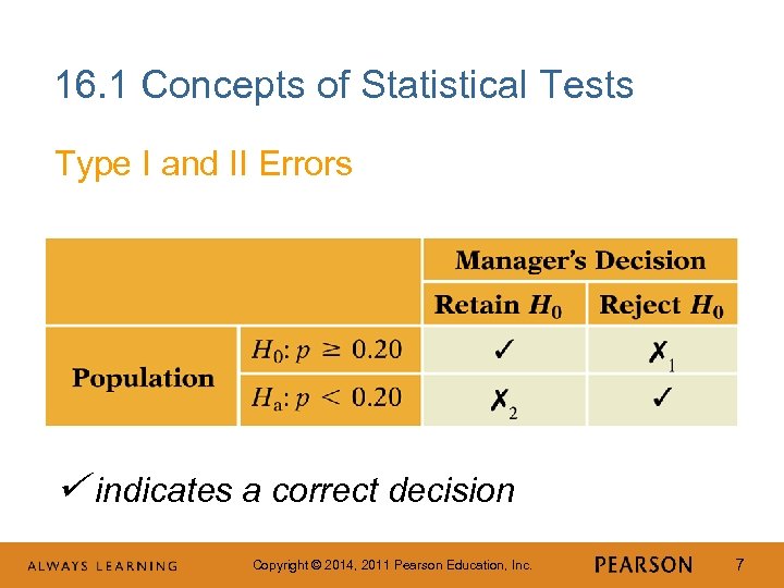 16. 1 Concepts of Statistical Tests Type I and II Errors indicates a correct decision Copyright © 2014, 2011 Pearson Education, Inc. 7
 16. 1 Concepts of Statistical Tests Other Tests § Visual inspection for association, normal quantile plots and control charts all use tests of hypotheses. § For example, the null hypothesis in a visual test for association is that there is no association between two variables shown in the scatterplot. Copyright © 2014, 2011 Pearson Education, Inc. 8
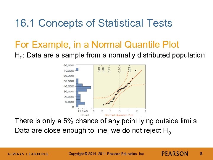 16. 1 Concepts of Statistical Tests For Example, in a Normal Quantile Plot H 0: Data are a sample from a normally distributed population There is only a 5% chance of any point lying outside limits. Data are close enough to line; we do not reject H 0 Copyright © 2014, 2011 Pearson Education, Inc. 9
 16. 1 Concepts of Statistical Tests Test Statistic § Statistical tests rely on the sampling distribution of the test statistic that estimates the parameter specified in the null and alternative hypotheses. § Key question: What is the chance of getting a test statistic this far from H 0 if H 0 is true? Copyright © 2014, 2011 Pearson Education, Inc. 10
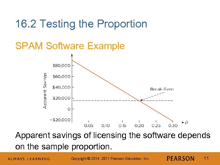 16. 2 Testing the Proportion SPAM Software Example Apparent savings of licensing the software depends on the sample proportion. Copyright © 2014, 2011 Pearson Education, Inc. 11
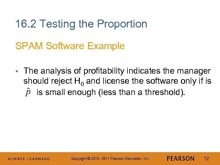 16. 2 Testing the Proportion SPAM Software Example § The analysis of profitability indicates the manager should reject H 0 and license the software only if is is small enough (less than a threshold). Copyright © 2014, 2011 Pearson Education, Inc. 12
 16. 2 Testing the Proportion SPAM Software Example α Level § The threshold for rejecting H 0 depends on manager’s willingness to take a chance on licensing software that won’t be profitable § Based on the probability of making a Type I error (designated as α – level of significance) Copyright © 2014, 2011 Pearson Education, Inc. 13
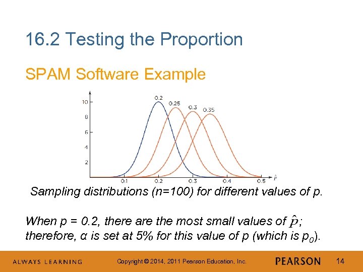 16. 2 Testing the Proportion SPAM Software Example Sampling distributions (n=100) for different values of p. When p = 0. 2, there are the most small values of ; therefore, α is set at 5% for this value of p (which is p 0). Copyright © 2014, 2011 Pearson Education, Inc. 14
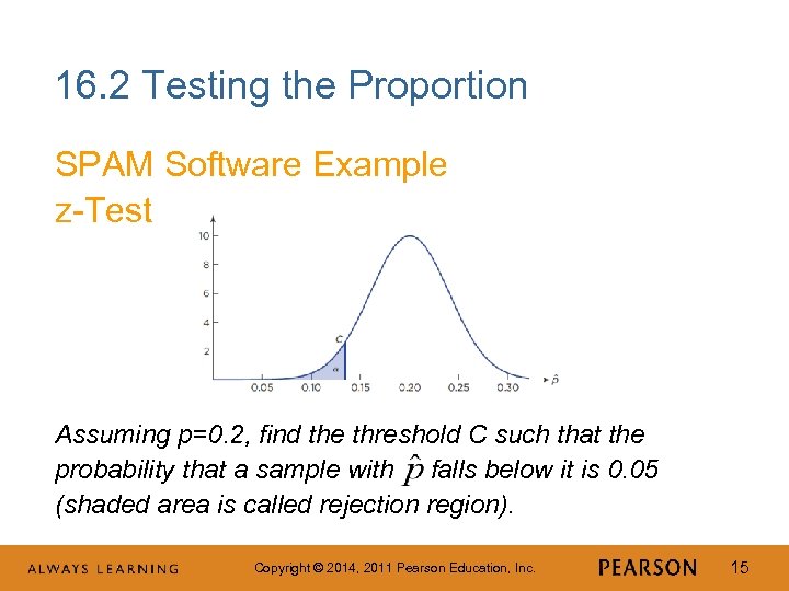 16. 2 Testing the Proportion SPAM Software Example z-Test Assuming p=0. 2, find the threshold C such that the probability that a sample with falls below it is 0. 05 (shaded area is called rejection region). Copyright © 2014, 2011 Pearson Education, Inc. 15
 16. 2 Testing the Proportion SPAM Software Example z-Test § P (Z < -1. 645) = 0. 05 § Based on n=100 and SE( ) = 0. 04 (note that the hypothesized value p 0 = 0. 20 is used to calculate SE), then C = 0. 2 – 1. 645 (0. 04) =. 01342. Copyright © 2014, 2011 Pearson Education, Inc. 16
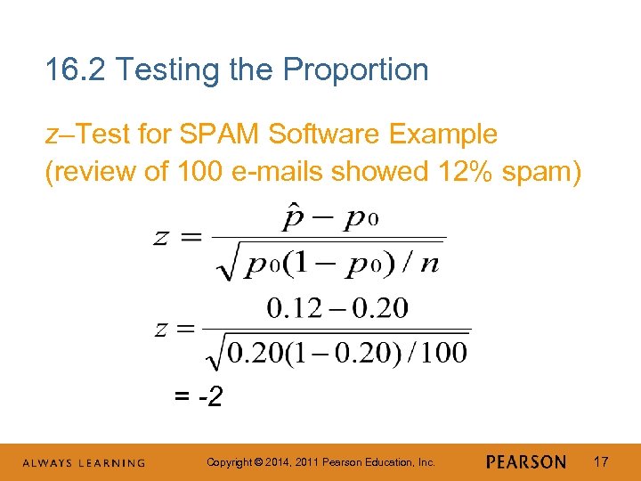 16. 2 Testing the Proportion z–Test for SPAM Software Example (review of 100 e-mails showed 12% spam) = -2 Copyright © 2014, 2011 Pearson Education, Inc. 17
 16. 2 Testing the Proportion SPAM Software Example § z-Test: test of H 0 based on a count of the standard errors separating H 0 from the test statistic. § The observed sample proportion is 2 standard errors below p 0. Since z < -1. 645 the managers rejects H 0; the result is statistically significant. Copyright © 2014, 2011 Pearson Education, Inc. 18
 16. 2 Testing the Proportion SPAM Software Example § p-Value: the smallest α level at which H 0 can be rejected. § Statistical software commonly reports the p-value of a test. Copyright © 2014, 2011 Pearson Education, Inc. 19
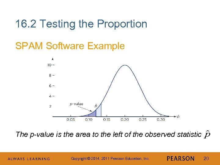 16. 2 Testing the Proportion SPAM Software Example The p-value is the area to the left of the observed statistic Copyright © 2014, 2011 Pearson Education, Inc. 20
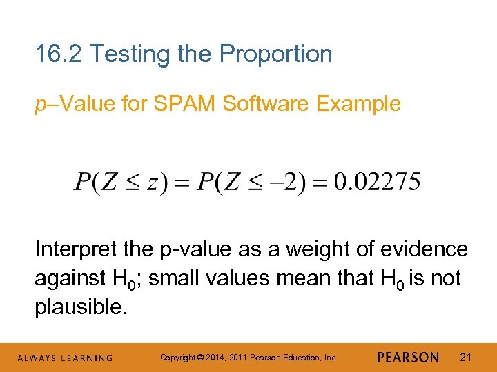 16. 2 Testing the Proportion p–Value for SPAM Software Example Interpret the p-value as a weight of evidence against H 0; small values mean that H 0 is not plausible. Copyright © 2014, 2011 Pearson Education, Inc. 21
 16. 2 Testing the Proportion p–Value for SPAM Software Example § Statistically significant: data contradict the null hypothesis and lead us to reject H 0 (p-value < α). § The p-value in the SPAM example is less than the typical α of 0. 05; should buy the software. Copyright © 2014, 2011 Pearson Education, Inc. 22
 16. 2 Testing the Proportion Type II Error § Power: probability that a test can reject H 0. § If a test has little power when H 0 is false, it is likely to miss meaningful deviations from the null hypothesis and produce a Type II error. Copyright © 2014, 2011 Pearson Education, Inc. 23
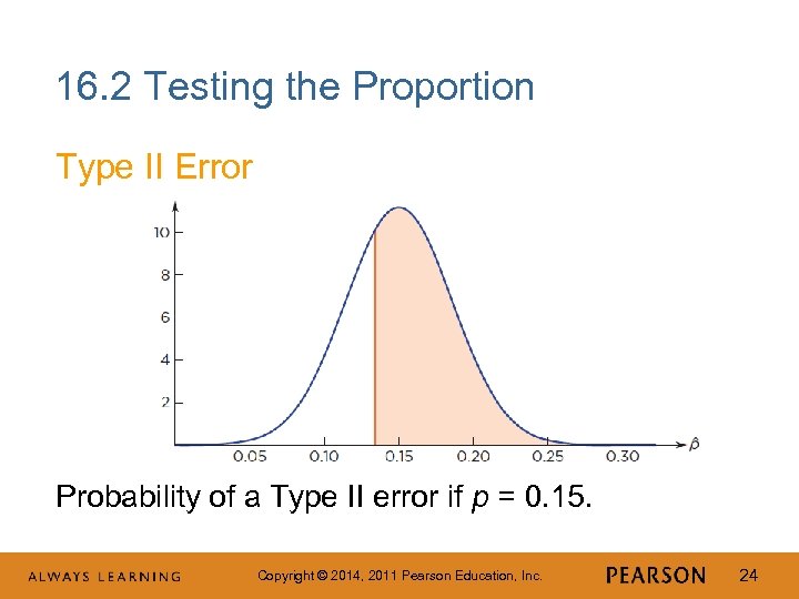 16. 2 Testing the Proportion Type II Error Probability of a Type II error if p = 0. 15. Copyright © 2014, 2011 Pearson Education, Inc. 24
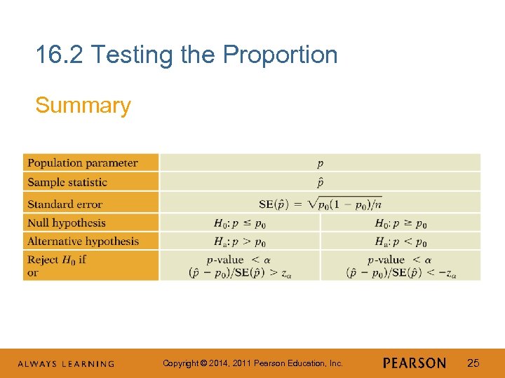 16. 2 Testing the Proportion Summary Copyright © 2014, 2011 Pearson Education, Inc. 25
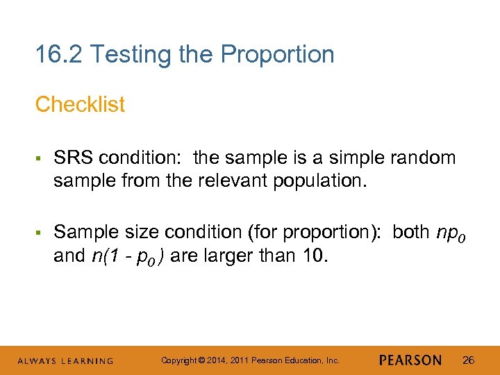 16. 2 Testing the Proportion Checklist § SRS condition: the sample is a simple random sample from the relevant population. § Sample size condition (for proportion): both np 0 and n(1 - p 0 ) are larger than 10. Copyright © 2014, 2011 Pearson Education, Inc. 26
 4 M Example 16. 1: DO ENOUGH HOUSEHOLDS WATCH? Motivation The Burger King ad featuring Coq Roq won critical acclaim. In a sample of 2, 500 homes, Media. Check found that only 6% saw the ad. An ad must be viewed by 5% or more of households to be effective. Based on these sample results, should the local sponsor run this ad? Copyright © 2014, 2011 Pearson Education, Inc. 27
 4 M Example 16. 1: DO ENOUGH HOUSEHOLDS WATCH? Method Set up the null and alternative hypotheses. H 0: p ≤ 0. 05 Ha: p > 0. 05 Use α = 0. 05. Note that p is the population proportion who watch this ad. Both SRS and sample size conditions are met. Copyright © 2014, 2011 Pearson Education, Inc. 28
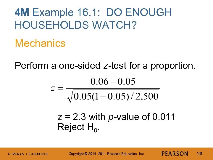 4 M Example 16. 1: DO ENOUGH HOUSEHOLDS WATCH? Mechanics Perform a one-sided z-test for a proportion. z = 2. 3 with p-value of 0. 011 Reject H 0. Copyright © 2014, 2011 Pearson Education, Inc. 29
 4 M Example 16. 1: DO ENOUGH HOUSEHOLDS WATCH? Message The results are statistically significant. We can conclude that more than 5% of households watch this ad. The Burger King Coq Roq ad is cost effective and should be run. Copyright © 2014, 2011 Pearson Education, Inc. 30
 16. 3 Testing the Mean Similar to Tests of Proportions § The hypothesis test of µ replaces § Unlike the test of proportions, σ is not specified. Use s from the sample as an estimate of σ to calculate the estimated standard error of. Copyright © 2014, 2011 Pearson Education, Inc. with . 31
 16. 3 Testing the Mean Example: San Francisco Rental Properties A firm is considering expanding into an expensive area in downtown San Francisco. In order to cover costs, the firm needs rents in this area to average more than $1, 500 per month. Are rents in San Francisco high enough to justify the expansion? Copyright © 2014, 2011 Pearson Education, Inc. 32
 16. 3 Testing the Mean Null and Alternative Hypotheses § Let µ = mean monthly rent for all rental properties in the San Francisco area § Set up hypotheses as: H 0: µ ≤ µ 0 = $1, 500 Ha: µ > µ 0 = $1, 500 Copyright © 2014, 2011 Pearson Education, Inc. 33
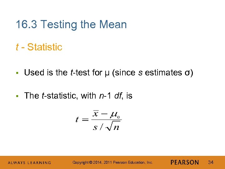 16. 3 Testing the Mean t - Statistic § Used is the t-test for µ (since s estimates σ) § The t-statistic, with n-1 df, is Copyright © 2014, 2011 Pearson Education, Inc. 34
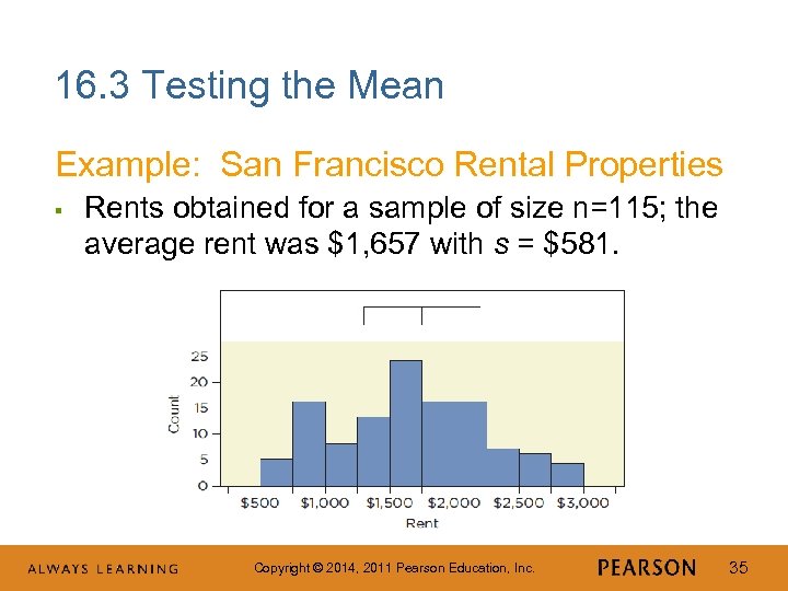 16. 3 Testing the Mean Example: San Francisco Rental Properties § Rents obtained for a sample of size n=115; the average rent was $1, 657 with s = $581. Copyright © 2014, 2011 Pearson Education, Inc. 35
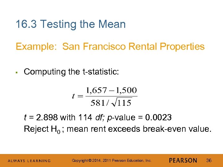 16. 3 Testing the Mean Example: San Francisco Rental Properties § Computing the t-statistic: t = 2. 898 with 114 df; p-value = 0. 0023 Reject H 0 ; mean rent exceeds break-even value. Copyright © 2014, 2011 Pearson Education, Inc. 36
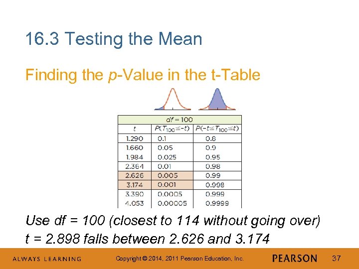 16. 3 Testing the Mean Finding the p-Value in the t-Table Use df = 100 (closest to 114 without going over) t = 2. 898 falls between 2. 626 and 3. 174 Copyright © 2014, 2011 Pearson Education, Inc. 37
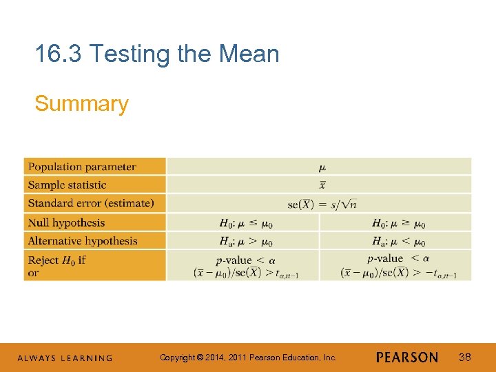 16. 3 Testing the Mean Summary Copyright © 2014, 2011 Pearson Education, Inc. 38
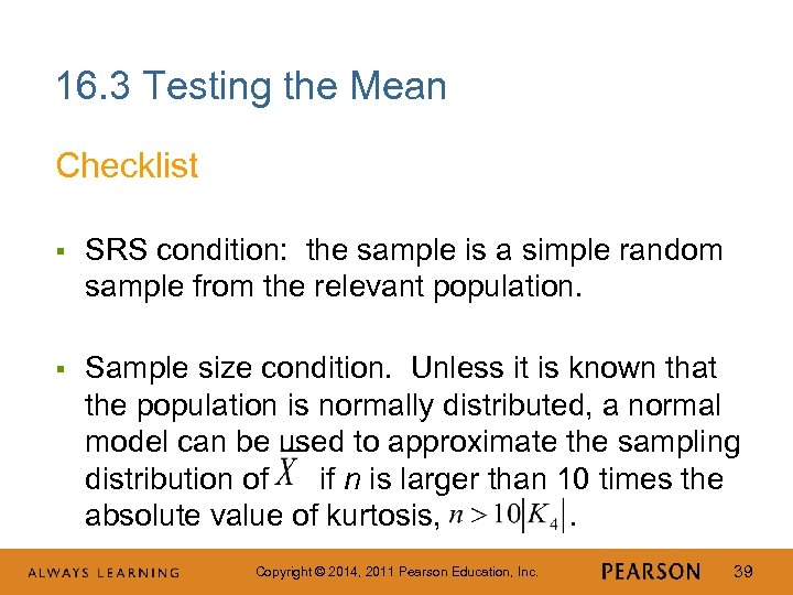 16. 3 Testing the Mean Checklist § SRS condition: the sample is a simple random sample from the relevant population. § Sample size condition. Unless it is known that the population is normally distributed, a normal model can be used to approximate the sampling distribution of if n is larger than 10 times the absolute value of kurtosis, . Copyright © 2014, 2011 Pearson Education, Inc. 39
 4 M Example 16. 2: COMPARING RETURNS ON INVESTMENTS Motivation Does stock in IBM return more, on average, than T-Bills? From 1990 through 2011, TBills returned 0. 3% each month. Copyright © 2014, 2011 Pearson Education, Inc. 40
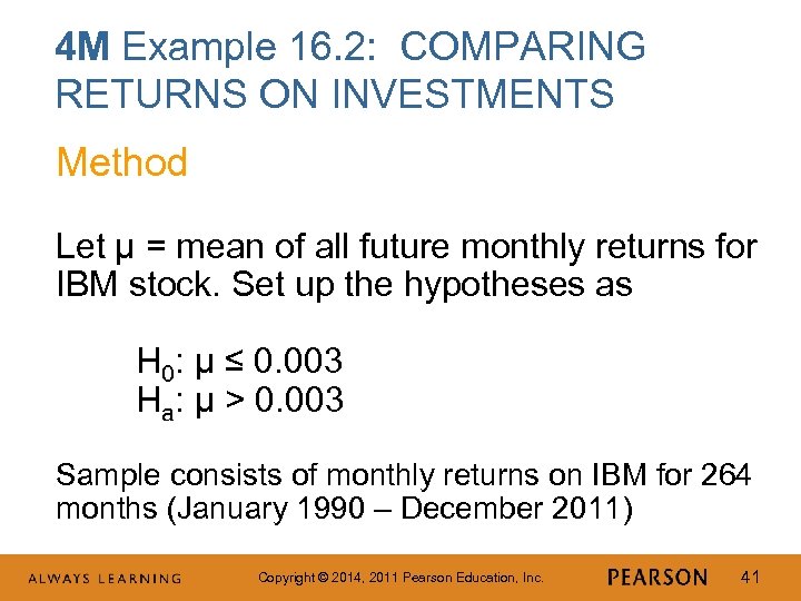 4 M Example 16. 2: COMPARING RETURNS ON INVESTMENTS Method Let µ = mean of all future monthly returns for IBM stock. Set up the hypotheses as H 0: µ ≤ 0. 003 Ha: µ > 0. 003 Sample consists of monthly returns on IBM for 264 months (January 1990 – December 2011) Copyright © 2014, 2011 Pearson Education, Inc. 41
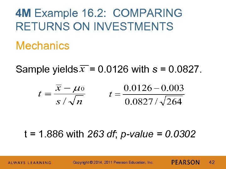 4 M Example 16. 2: COMPARING RETURNS ON INVESTMENTS Mechanics Sample yields = 0. 0126 with s = 0. 0827. t = 1. 886 with 263 df; p-value = 0. 0302 Copyright © 2014, 2011 Pearson Education, Inc. 42
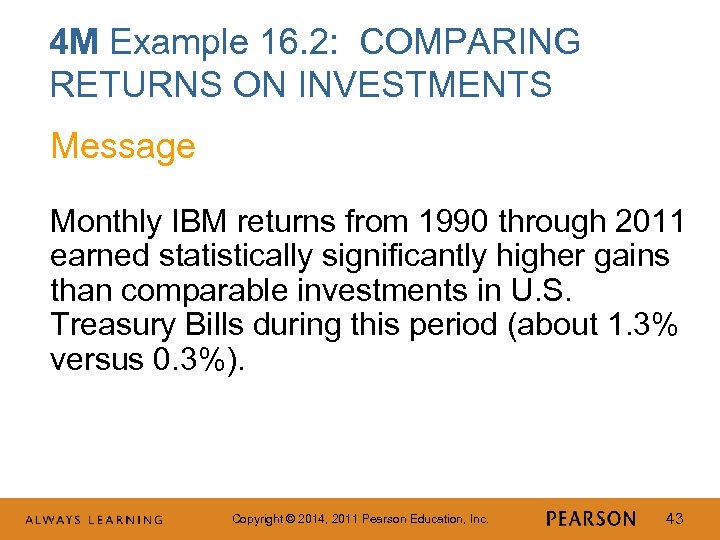 4 M Example 16. 2: COMPARING RETURNS ON INVESTMENTS Message Monthly IBM returns from 1990 through 2011 earned statistically significantly higher gains than comparable investments in U. S. Treasury Bills during this period (about 1. 3% versus 0. 3%). Copyright © 2014, 2011 Pearson Education, Inc. 43
 16. 4 Significance vs Importance § Statistical significance does not mean that you have made an important or meaningful discovery. § The size of the sample affects the p-value of a test. With enough data, a trivial difference from H 0 leads to a statistically significant outcome. Copyright © 2014, 2011 Pearson Education, Inc. 44
 16. 5 Confidence Interval or Test? § A confidence interval provides a range of parameter values that are compatible with the observed data. § A test provides a precise analysis of a specific hypothesized value for a parameter. § Most people understand the implications of confidence intervals more readily than tests. Copyright © 2014, 2011 Pearson Education, Inc. 45
 Best Practices § Pick the hypotheses before looking at the data. § Choose the null hypothesis on the basis of profitability. § Pick the α-level first, taking into account both types of error. § Think about whether α = 0. 05 is appropriate for each test. Copyright © 2014, 2011 Pearson Education, Inc. 46
 Best Practices (Continued) § Make sure to have an SRS from the right population. § Use a one-sided test. § Report a p–value to summarize the outcome of a test. Copyright © 2014, 2011 Pearson Education, Inc. 47
 Pitfalls § Do not confuse statistical significance with substantive importance. § Do not think that the p–value is the probability that the null hypothesis is true. § Avoid cluttering a test summary with jargon. Copyright © 2014, 2011 Pearson Education, Inc. 48


