010d9980dda8720ff8242741355b3ade.ppt
- Количество слайдов: 146
 Chapter 15 Nonparametric Statistics © 2010 Pearson Prentice Hall. All rights reserved
 Section 15. 1 An Overview of Nonparametric Statistics © 2010 Pearson Prentice Hall. All rights reserved
 Objective 1. Understand the difference between parametric statistical procedures and nonparametric statistical procedures © 2010 Pearson Prentice Hall. All rights reserved 104
 Parametric statistical procedures are inferential procedures conducted under the assumption that the underlying distribution of the data belongs to some parametric family of distributions (such as the normal distribution). © 2010 Pearson Prentice Hall. All rights reserved 105
 Nonparametric statistical procedures are inferential procedures that do not make any assumptions about the underlying distribution of the data. They do not require that the population belong to any particular parametric family of distributions (such as the normal distribution) and, therefore, are often referred to as distributionfree procedures. © 2010 Pearson Prentice Hall. All rights reserved 106
 Advantages of Nonparametric Statistical Procedures • Most of the tests have very few requirements, so it is unlikely that these tests will be used improperly. © 2010 Pearson Prentice Hall. All rights reserved 107
 Advantages of Nonparametric Statistical Procedures • Most of the tests have very few requirements, so it is unlikely that these tests will be used improperly. • For some nonparametric procedures, the computations are fairly easy. © 2010 Pearson Prentice Hall. All rights reserved 108
 Advantages of Nonparametric Statistical Procedures • Most of the tests have very few requirements, so it is unlikely that these tests will be used improperly. • For some nonparametric procedures, the computations are fairly easy. • The procedures can be used for count data or rank data, so nonparametric methods can be used on data, such as the rankings of a movie as excellent, good, fair, or poor. © 2010 Pearson Prentice Hall. All rights reserved 109
 Disadvantages of Nonparametric Statistical Procedures • Nonparametric procedures are less efficient than parametric procedures. This means that a larger sample size is required when conducting a nonparametric procedure to have the same probability of a Type I error as the equivalent parametric procedure. © 2010 Pearson Prentice Hall. All rights reserved 110
 Disadvantages of Nonparametric Statistical Procedures • Nonparametric procedures often discard useful information. For example, the sign test uses only the sign of the data and rank tests merely preserve orderthe magnitude of the actual data values is lost. As a result, nonparametric procedures are typically less powerful. Recall that the power of a test refers to the probability of making a Type II error. A Type II error occurs when a researcher does not reject the null hypothesis when the alternative hypothesis is true. © 2010 Pearson Prentice Hall. All rights reserved 111
 Disadvantages of Nonparametric Statistical Procedures • Because fewer requirements must be satisfied to conduct these tests, researchers sometimes use these procedures when parametric procedures can be used. © 2010 Pearson Prentice Hall. All rights reserved 112
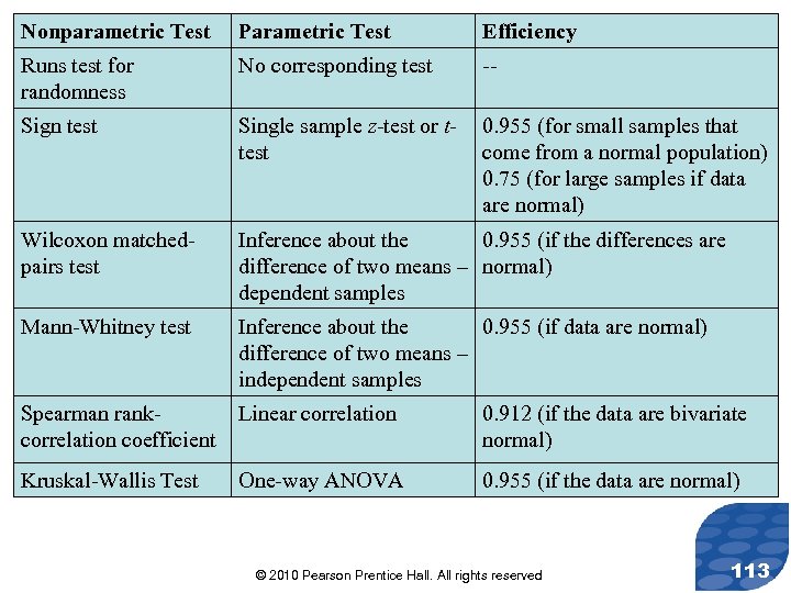 Nonparametric Test Parametric Test Efficiency Runs test for randomness No corresponding test -- Sign test Single sample z-test or ttest 0. 955 (for small samples that come from a normal population) 0. 75 (for large samples if data are normal) Wilcoxon matchedpairs test Inference about the 0. 955 (if the differences are difference of two means – normal) dependent samples Mann-Whitney test Inference about the 0. 955 (if data are normal) difference of two means – independent samples Spearman rankcorrelation coefficient Linear correlation 0. 912 (if the data are bivariate normal) Kruskal-Wallis Test One-way ANOVA 0. 955 (if the data are normal) © 2010 Pearson Prentice Hall. All rights reserved 113
 “In Other Words” The lower the efficiency is, the larger the sample size must be for a nonparametric test to have the probability of a Type I error the same as it would be for its equivalent parametric test. © 2010 Pearson Prentice Hall. All rights reserved 114
 Section 15. 2 Runs Test for Randomness © 2010 Pearson Prentice Hall. All rights reserved
 Objective 1. Perform a runs test for randomness © 2010 Pearson Prentice Hall. All rights reserved 116
 A runs test for randomness is used to test whether data have been obtained or occur randomly. A run is a sequence of similar events, items, or symbols that is followed by an event, item, or symbol that is mutually exclusive from the first event, item, or symbol. The number of events, items, or symbols in a run is called its length. © 2010 Pearson Prentice Hall. All rights reserved 117
 CAUTION! Runs tests are used to test whether it is reasonable to conclude that data occur randomly, not whether the data are collected randomly. For example, we might wonder whether defective parts come off an assembly line randomly or systematically. If broken parts occur systematically (such as every fourth part), we might be led to believe that we have a broken machine. We don’t collect the data randomly; instead, we select 100 consecutive parts. We want to know whether the defective parts in the 100 selected occur randomly. © 2010 Pearson Prentice Hall. All rights reserved 118
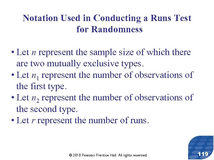 Notation Used in Conducting a Runs Test for Randomness • Let n represent the sample size of which there are two mutually exclusive types. • Let n 1 represent the number of observations of the first type. • Let n 2 represent the number of observations of the second type. • Let r represent the number of runs. © 2010 Pearson Prentice Hall. All rights reserved 119
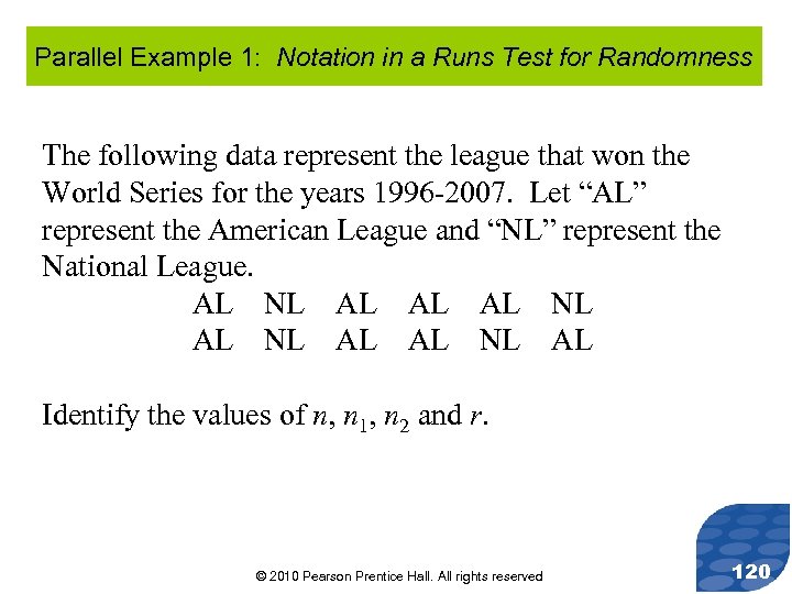 Parallel Example 1: Notation in a Runs Test for Randomness The following data represent the league that won the World Series for the years 1996 -2007. Let “AL” represent the American League and “NL” represent the National League. AL NL AL AL NL AL Identify the values of n, n 1, n 2 and r. © 2010 Pearson Prentice Hall. All rights reserved 120
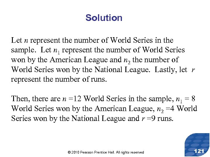 Solution Let n represent the number of World Series in the sample. Let n 1 represent the number of World Series won by the American League and n 2 the number of World Series won by the National League. Lastly, let r represent the number of runs. Then, there are n =12 World Series in the sample, n 1 = 8 World Series won by the American League, n 2 =4 World Series won by the National League and r =9 runs. © 2010 Pearson Prentice Hall. All rights reserved 121
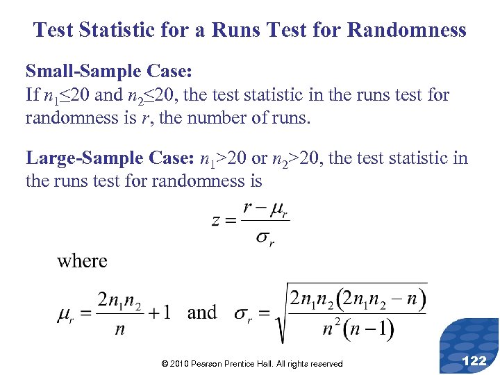 Test Statistic for a Runs Test for Randomness Small-Sample Case: If n 1≤ 20 and n 2≤ 20, the test statistic in the runs test for randomness is r, the number of runs. Large-Sample Case: n 1>20 or n 2>20, the test statistic in the runs test for randomness is © 2010 Pearson Prentice Hall. All rights reserved 122
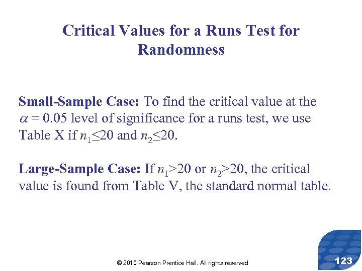 Critical Values for a Runs Test for Randomness Small-Sample Case: To find the critical value at the = 0. 05 level of significance for a runs test, we use Table X if n 1≤ 20 and n 2≤ 20. Large-Sample Case: If n 1>20 or n 2>20, the critical value is found from Table V, the standard normal table. © 2010 Pearson Prentice Hall. All rights reserved 123
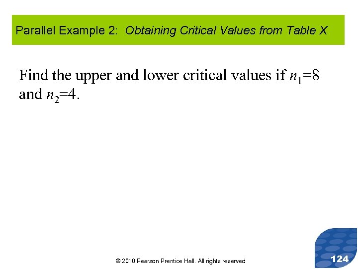 Parallel Example 2: Obtaining Critical Values from Table X Find the upper and lower critical values if n 1=8 and n 2=4. © 2010 Pearson Prentice Hall. All rights reserved 124
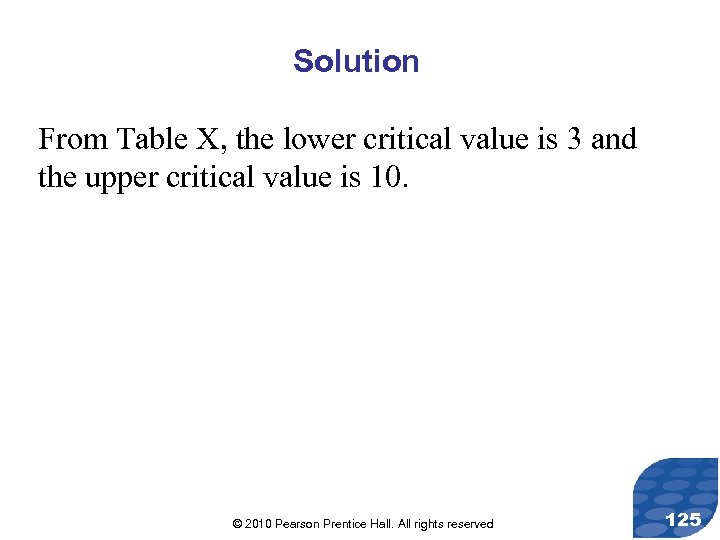 Solution From Table X, the lower critical value is 3 and the upper critical value is 10. © 2010 Pearson Prentice Hall. All rights reserved 125
 Runs Test for Randomness To test the randomness of data, we can use the following steps, provided that 1. the sample is a sequence of observations recorded in the order of their occurrence, and 2. the observations can be categorized into two mutually exclusive categories. © 2010 Pearson Prentice Hall. All rights reserved 126
 Step 1: Assume the data are random. This forms the basis of the null and alternative hypotheses, which are structured as follows: H 0: The sequence of data is random H 1: The sequence of data is not random © 2010 Pearson Prentice Hall. All rights reserved 127
 Step 2: Determine a level of significance, , based on the seriousness of making a Type I error. The level of significance is used to determine the critical value. Note: For the small-sample case, we must use the level of significance =0. 05. © 2010 Pearson Prentice Hall. All rights reserved 128
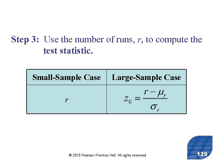 Step 3: Use the number of runs, r, to compute the test statistic. Small-Sample Case Large-Sample Case r © 2010 Pearson Prentice Hall. All rights reserved 129
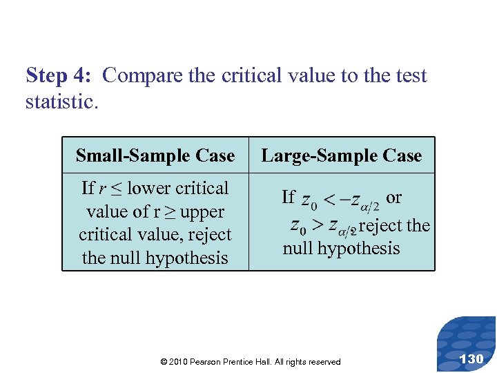 Step 4: Compare the critical value to the test statistic. Small-Sample Case If r ≤ lower critical value of r ≥ upper critical value, reject the null hypothesis Large-Sample Case If or , reject the null hypothesis © 2010 Pearson Prentice Hall. All rights reserved 130
 Step 5: State the conclusion. © 2010 Pearson Prentice Hall. All rights reserved 131
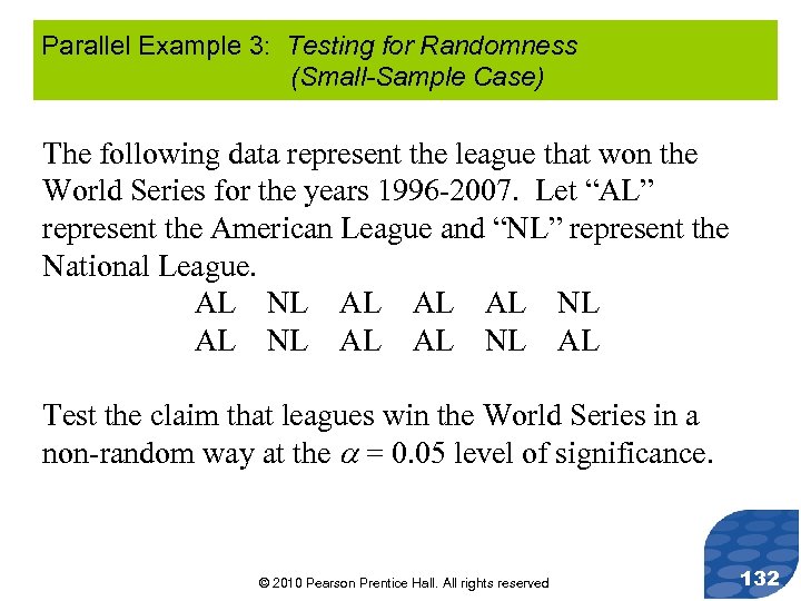 Parallel Example 3: Testing for Randomness (Small-Sample Case) The following data represent the league that won the World Series for the years 1996 -2007. Let “AL” represent the American League and “NL” represent the National League. AL NL AL AL NL AL Test the claim that leagues win the World Series in a non-random way at the = 0. 05 level of significance. © 2010 Pearson Prentice Hall. All rights reserved 132
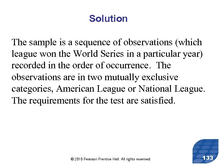 Solution The sample is a sequence of observations (which league won the World Series in a particular year) recorded in the order of occurrence. The observations are in two mutually exclusive categories, American League or National League. The requirements for the test are satisfied. © 2010 Pearson Prentice Hall. All rights reserved 133
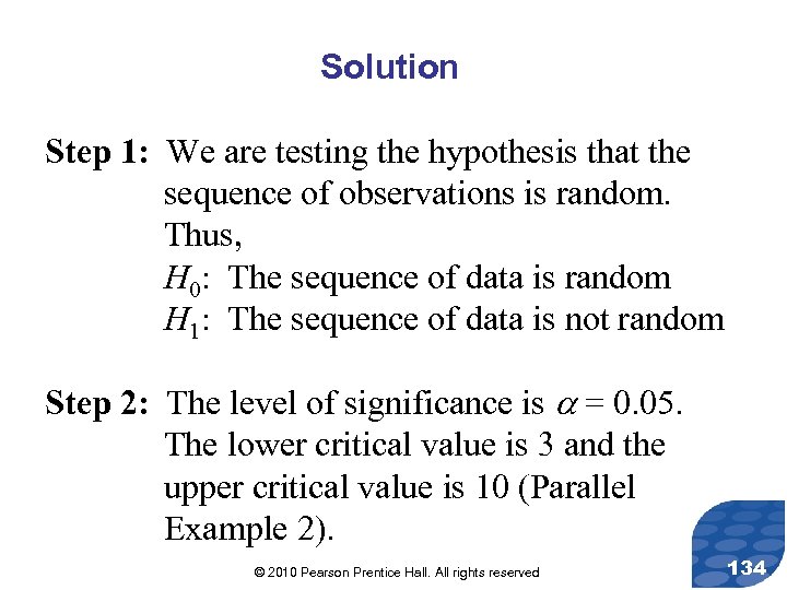 Solution Step 1: We are testing the hypothesis that the sequence of observations is random. Thus, H 0: The sequence of data is random H 1: The sequence of data is not random Step 2: The level of significance is = 0. 05. The lower critical value is 3 and the upper critical value is 10 (Parallel Example 2). © 2010 Pearson Prentice Hall. All rights reserved 134
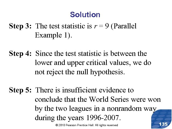 Solution Step 3: The test statistic is r = 9 (Parallel Example 1). Step 4: Since the test statistic is between the lower and upper critical values, we do not reject the null hypothesis. Step 5: There is insufficient evidence to conclude that the World Series were won by the two leagues in a nonrandom way during the years 1996 -2007. © 2010 Pearson Prentice Hall. All rights reserved 135
 Section 15. 3 Inferences About Measures of Central Tendency © 2010 Pearson Prentice Hall. All rights reserved
 Objective 1. Conduct a one-sample sign test © 2010 Pearson Prentice Hall. All rights reserved 137
 A one-sample sign test is a nonparametric test that uses data, converted to plus and minus signs, to test a hypothesis regarding the median of a population. Data values equal to the assumed value of the median are ignored during the test. © 2010 Pearson Prentice Hall. All rights reserved 138
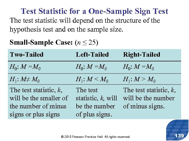 Test Statistic for a One-Sample Sign Test The test statistic will depend on the structure of the hypothesis test and on the sample size. Small-Sample Case: (n ≤ 25) Two-Tailed Left-Tailed Right-Tailed H 0: M =M 0 H 1: M≠ M 0 H 1: M < M 0 H 1: M > M 0 The test statistic, k, will be the smaller of the number of minus signs or plus signs The test statistic, k, will be the number of minus signs. of plus signs. © 2010 Pearson Prentice Hall. All rights reserved 139
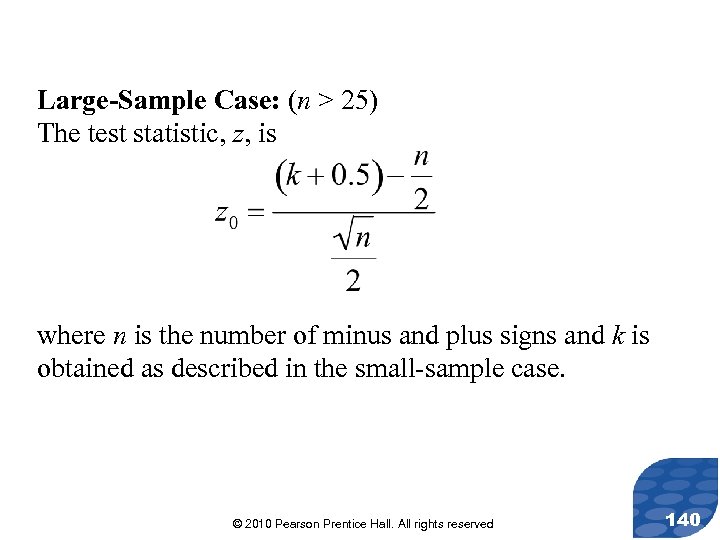 Large-Sample Case: (n > 25) The test statistic, z, is where n is the number of minus and plus signs and k is obtained as described in the small-sample case. © 2010 Pearson Prentice Hall. All rights reserved 140
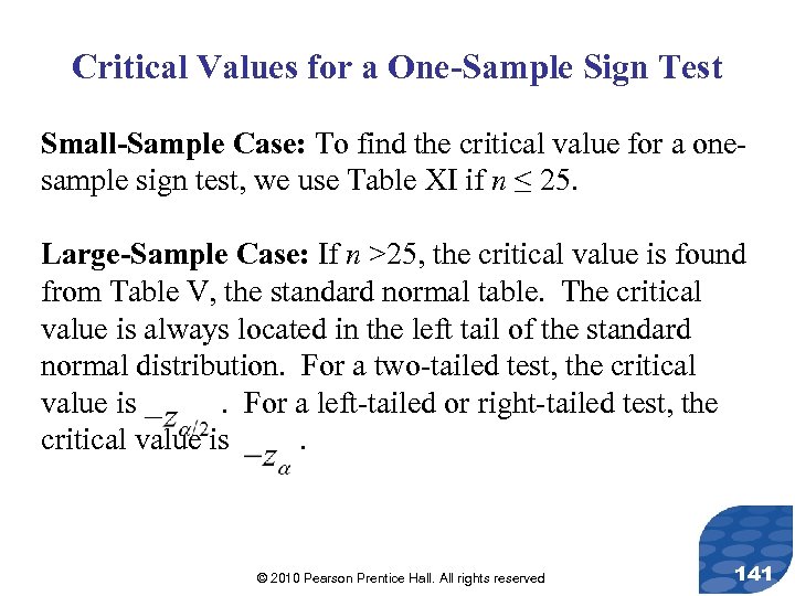 Critical Values for a One-Sample Sign Test Small-Sample Case: To find the critical value for a onesample sign test, we use Table XI if n ≤ 25. Large-Sample Case: If n >25, the critical value is found from Table V, the standard normal table. The critical value is always located in the left tail of the standard normal distribution. For a two-tailed test, the critical value is. For a left-tailed or right-tailed test, the critical value is. © 2010 Pearson Prentice Hall. All rights reserved 141
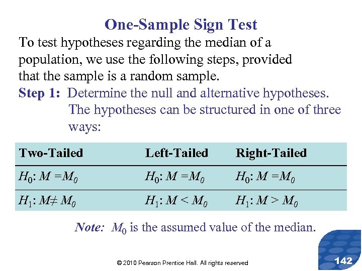 One-Sample Sign Test To test hypotheses regarding the median of a population, we use the following steps, provided that the sample is a random sample. Step 1: Determine the null and alternative hypotheses. The hypotheses can be structured in one of three ways: Two-Tailed Left-Tailed Right-Tailed H 0: M =M 0 H 1: M≠ M 0 H 1: M < M 0 H 1: M > M 0 Note: M 0 is the assumed value of the median. © 2010 Pearson Prentice Hall. All rights reserved 142
 Step 2: Count the number of observations below M 0, and assign them minus (-) signs. Count the number of observations above M 0, and assign them plus (+) signs. © 2010 Pearson Prentice Hall. All rights reserved 143
 Step 3: Select a level of significance, , based on the seriousness of making a Type I error. The level of significance is used to determine the critical value. The critical value for small samples (n ≤ 25) is found from Table XI. The critical value for large samples (n > 25) is found from Table V. © 2010 Pearson Prentice Hall. All rights reserved 144
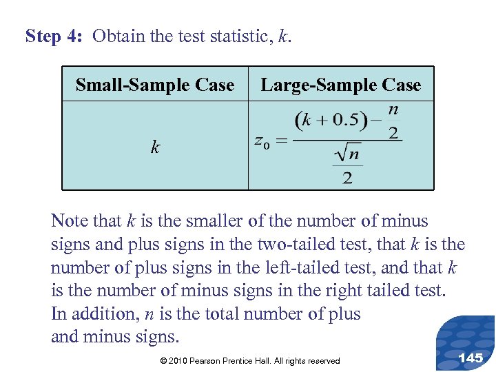 Step 4: Obtain the test statistic, k. Small-Sample Case Large-Sample Case k Note that k is the smaller of the number of minus signs and plus signs in the two-tailed test, that k is the number of plus signs in the left-tailed test, and that k is the number of minus signs in the right tailed test. In addition, n is the total number of plus and minus signs. © 2010 Pearson Prentice Hall. All rights reserved 145
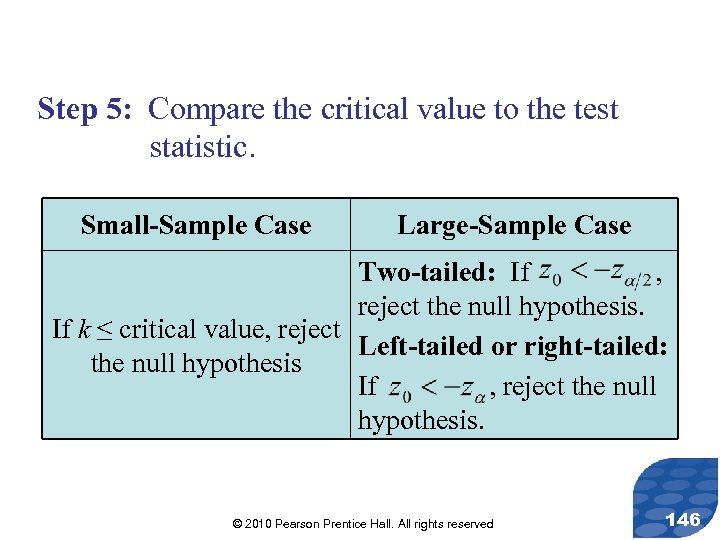 Step 5: Compare the critical value to the test statistic. Small-Sample Case Large-Sample Case Two-tailed: If , reject the null hypothesis. If k ≤ critical value, reject Left-tailed or right-tailed: the null hypothesis If , reject the null hypothesis. © 2010 Pearson Prentice Hall. All rights reserved 146
 Step 6: State the conclusion. © 2010 Pearson Prentice Hall. All rights reserved 147
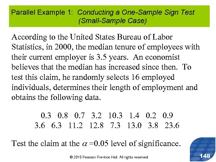 Parallel Example 1: Conducting a One-Sample Sign Test (Small-Sample Case) According to the United States Bureau of Labor Statistics, in 2000, the median tenure of employees with their current employer is 3. 5 years. An economist believes that the median has increased since then. To test this claim, he randomly selects 16 employed individuals, determines their length of employment and obtains the following data. 0. 3 0. 8 0. 7 3. 2 10. 3 1. 4 0. 2 0. 9 3. 6 6. 3 11. 2 12. 8 7. 3 13. 0 3. 8 23. 6 Test the claim at the =0. 05 level of significance. © 2010 Pearson Prentice Hall. All rights reserved 148
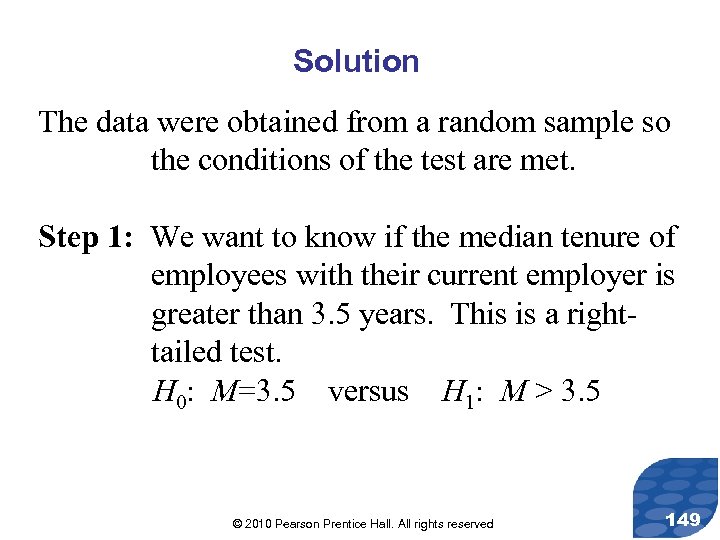 Solution The data were obtained from a random sample so the conditions of the test are met. Step 1: We want to know if the median tenure of employees with their current employer is greater than 3. 5 years. This is a righttailed test. H 0: M=3. 5 versus H 1: M > 3. 5 © 2010 Pearson Prentice Hall. All rights reserved 149
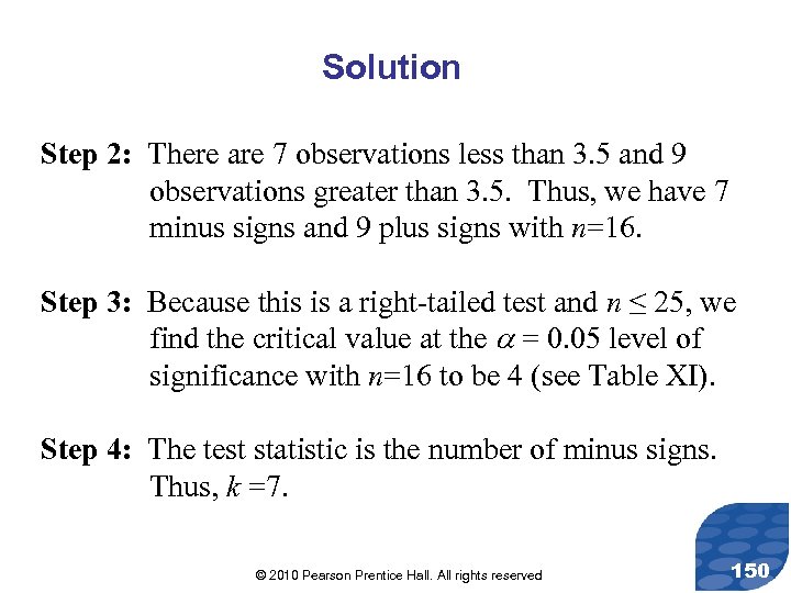 Solution Step 2: There are 7 observations less than 3. 5 and 9 observations greater than 3. 5. Thus, we have 7 minus signs and 9 plus signs with n=16. Step 3: Because this is a right-tailed test and n ≤ 25, we find the critical value at the = 0. 05 level of significance with n=16 to be 4 (see Table XI). Step 4: The test statistic is the number of minus signs. Thus, k =7. © 2010 Pearson Prentice Hall. All rights reserved 150
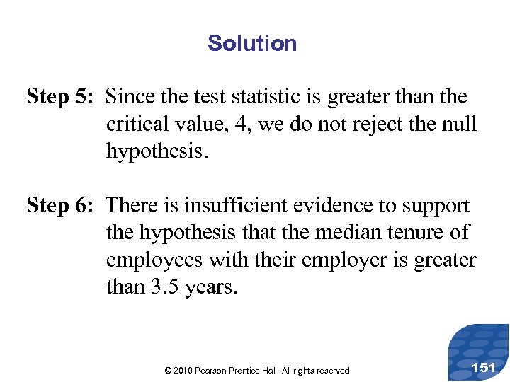 Solution Step 5: Since the test statistic is greater than the critical value, 4, we do not reject the null hypothesis. Step 6: There is insufficient evidence to support the hypothesis that the median tenure of employees with their employer is greater than 3. 5 years. © 2010 Pearson Prentice Hall. All rights reserved 151
 Section 15. 4 Inferences About The Difference Between Two Medians: Dependent Samples © 2010 Pearson Prentice Hall. All rights reserved
 Objective 1. Test a hypothesis about the difference between the medians of two dependent samples © 2010 Pearson Prentice Hall. All rights reserved 153
 The Wilcoxon Matched-Pairs Signed-Ranks Test is a nonparametric procedure used to test the equality of two population medians by dependent sampling. © 2010 Pearson Prentice Hall. All rights reserved 154
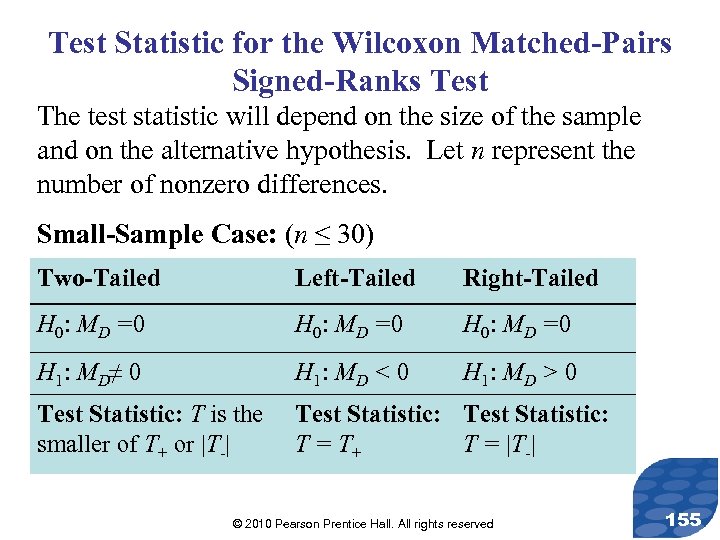 Test Statistic for the Wilcoxon Matched-Pairs Signed-Ranks Test The test statistic will depend on the size of the sample and on the alternative hypothesis. Let n represent the number of nonzero differences. Small-Sample Case: (n ≤ 30) Two-Tailed Left-Tailed Right-Tailed H 0: MD =0 H 1: MD≠ 0 H 1: MD < 0 H 1: MD > 0 Test Statistic: T is the smaller of T+ or |T-| Test Statistic: T = T+ T = |T-| © 2010 Pearson Prentice Hall. All rights reserved 155
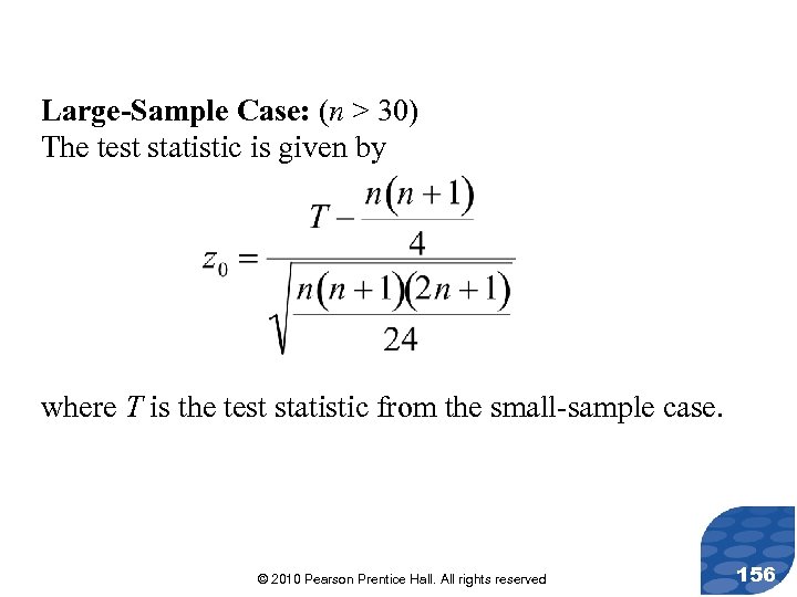 Large-Sample Case: (n > 30) The test statistic is given by where T is the test statistic from the small-sample case. © 2010 Pearson Prentice Hall. All rights reserved 156
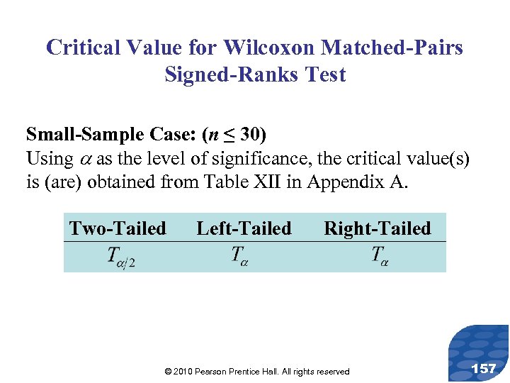 Critical Value for Wilcoxon Matched-Pairs Signed-Ranks Test Small-Sample Case: (n ≤ 30) Using as the level of significance, the critical value(s) is (are) obtained from Table XII in Appendix A. Two-Tailed Left-Tailed Right-Tailed © 2010 Pearson Prentice Hall. All rights reserved 157
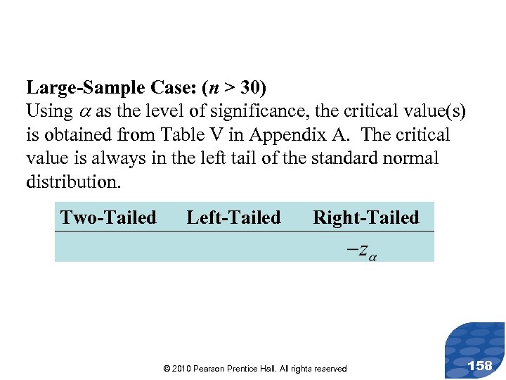 Large-Sample Case: (n > 30) Using as the level of significance, the critical value(s) is obtained from Table V in Appendix A. The critical value is always in the left tail of the standard normal distribution. Two-Tailed Left-Tailed Right-Tailed © 2010 Pearson Prentice Hall. All rights reserved 158
 Wilcoxon Matched-Pairs Signed-Ranks Test If a hypothesis is made regarding the medians of two populations, we can use the following steps to test the hypothesis, provided that 1. the samples are dependent random samples and 2. the distribution of the differences is symmetric. Although tests for verifying the symmetry of data exist, we do not present them in this text. All the data given satisfy the second requirement. © 2010 Pearson Prentice Hall. All rights reserved 159
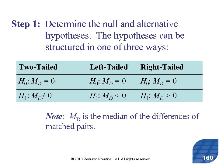 Step 1: Determine the null and alternative hypotheses. The hypotheses can be structured in one of three ways: Two-Tailed Left-Tailed Right-Tailed H 0: MD = 0 H 1: MD≠ 0 H 1: MD < 0 H 1: MD > 0 Note: MD is the median of the differences of matched pairs. © 2010 Pearson Prentice Hall. All rights reserved 160
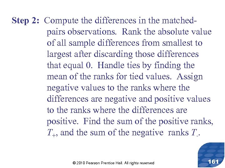 Step 2: Compute the differences in the matchedpairs observations. Rank the absolute value of all sample differences from smallest to largest after discarding those differences that equal 0. Handle ties by finding the mean of the ranks for tied values. Assign negative values to the ranks where the differences are negative and positive values to the ranks where the differences are positive. Find the sum of the positive ranks, T+, and the sum of the negative ranks T-. © 2010 Pearson Prentice Hall. All rights reserved 161
 Step 3: Draw a boxplot of the differences to compare the sample data from the two populations. This helps to visualize the difference in the medians. © 2010 Pearson Prentice Hall. All rights reserved 162
 Step 4: Choose a level of significance, , based on the seriousness of making a Type I error. The level of significance is used to determine the critical value. The critical value is found from Table XII for small samples (n ≤ 30). The critical value is found from Table V for large samples (n > 30). © 2010 Pearson Prentice Hall. All rights reserved 163
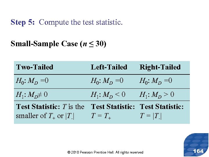 Step 5: Compute the test statistic. Small-Sample Case (n ≤ 30) Two-Tailed Left-Tailed Right-Tailed H 0: MD =0 H 1: MD≠ 0 H 1: MD < 0 H 1: MD > 0 Test Statistic: T is the Test Statistic: smaller of T+ or |T-| T = T+ T = |T-| © 2010 Pearson Prentice Hall. All rights reserved 164
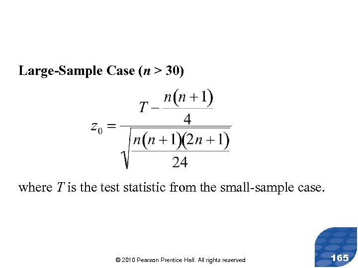 Large-Sample Case (n > 30) where T is the test statistic from the small-sample case. © 2010 Pearson Prentice Hall. All rights reserved 165
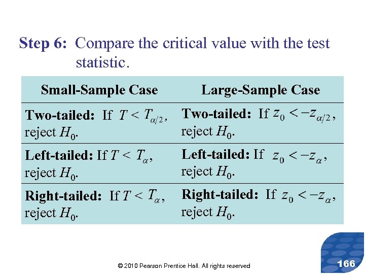 Step 6: Compare the critical value with the test statistic. Small-Sample Case , Two-tailed: If reject H 0. Two-tailed: If T < reject H 0. Left-tailed: If T < reject H 0. Right-tailed: If T < reject H 0. Large-Sample Case Left-tailed: If reject H 0. , , Right-tailed: If reject H 0. © 2010 Pearson Prentice Hall. All rights reserved , , , 166
 Step 7: State the conclusion. © 2010 Pearson Prentice Hall. All rights reserved 167
 Parallel Example 1: Wilcoxon Matched-Pairs Signed-Ranks Test (Small-Sample Case) The data on the following slide represent the cost of a one night stay in Hampton Inn Hotels and La Quinta Inn Hotels for a random sample of 10 cities. Test the claim that Hampton Inn Hotels are priced differently than La Quinta Hotels at the =0. 05 level of significance. © 2010 Pearson Prentice Hall. All rights reserved 168
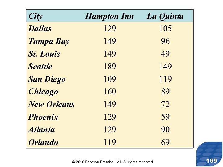 City Dallas Tampa Bay St. Louis Seattle San Diego Chicago New Orleans Phoenix Atlanta Orlando Hampton Inn 129 149 189 109 160 149 129 119 La Quinta 105 96 49 119 89 72 59 90 69 © 2010 Pearson Prentice Hall. All rights reserved 169
 Solution The data were obtained randomly. We assume that the symmetry requirement is satisfied. Step 1: We want to know if the hotels are priced differently. This is a two-tailed test. H 0: MD =0 versus H 1: MD ≠ 0 © 2010 Pearson Prentice Hall. All rights reserved 170
 Solution Step 2: In order to calculate T+ and T-, we must find the differences, rank them, and then attach the sign of the difference to the ranks. The differences and their signed ranks are given in the next slide. © 2010 Pearson Prentice Hall. All rights reserved 171
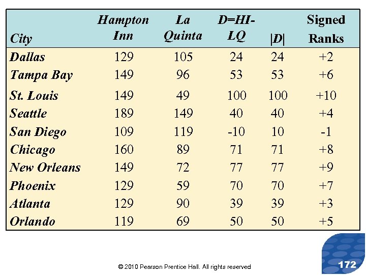 City Dallas Tampa Bay St. Louis Seattle San Diego Chicago New Orleans Phoenix Atlanta Orlando Hampton Inn La Quinta D=HILQ 24 53 |D| 24 53 Signed Ranks +2 +6 129 149 105 96 149 189 109 160 149 129 119 49 119 89 72 59 90 69 100 40 -10 71 77 70 39 50 100 40 10 71 77 70 39 50 +10 +4 -1 +8 +9 +7 +3 +5 © 2010 Pearson Prentice Hall. All rights reserved 172
 Solution Step 2: From the previous slide, we find that T+=54 and |T-| = 1. © 2010 Pearson Prentice Hall. All rights reserved 173
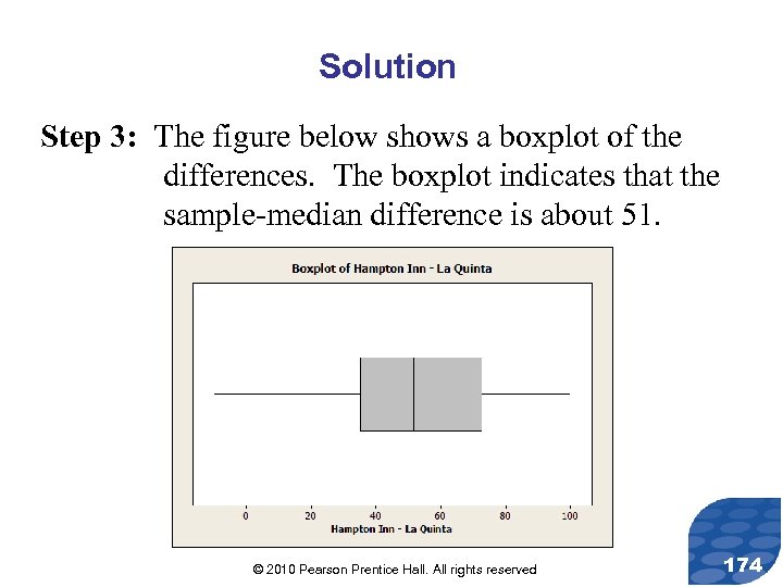 Solution Step 3: The figure below shows a boxplot of the differences. The boxplot indicates that the sample-median difference is about 51. © 2010 Pearson Prentice Hall. All rights reserved 174
 Solution Step 4: We are testing the hypothesis at the =0. 05 level of significance. Since this is a two-tailed test and the sample size is less than 30, we find the critical value with n=10 by using Table XII and obtain T 0. 025=8. Step 5: The test statistic is the smaller of T+ and |T-| which is 1. © 2010 Pearson Prentice Hall. All rights reserved 175
 Solution Step 6: The test statistic is less than the critical value (1< 8), so we reject the null hypothesis. Step 7: There is sufficient evidence at the =0. 05 level of significance to conclude that the median room price at Hampton Inns is different than the median room price at La Quinta Inns. © 2010 Pearson Prentice Hall. All rights reserved 176
 Section 15. 5 Inferences About The Difference Between Two Medians: Independent Samples © 2010 Pearson Prentice Hall. All rights reserved
 Objective 1. Test a hypothesis about the difference between the medians of two independent samples © 2010 Pearson Prentice Hall. All rights reserved 178
 The Mann-Whitney Test is a nonparametric procedure that is used to test the equality of two population medians from independent samples. © 2010 Pearson Prentice Hall. All rights reserved 179
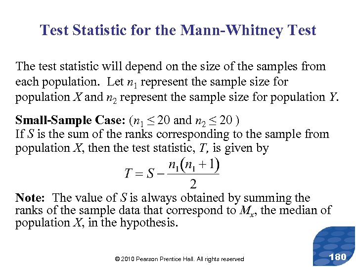 Test Statistic for the Mann-Whitney Test The test statistic will depend on the size of the samples from each population. Let n 1 represent the sample size for population X and n 2 represent the sample size for population Y. Small-Sample Case: (n 1 ≤ 20 and n 2 ≤ 20 ) If S is the sum of the ranks corresponding to the sample from population X, then the test statistic, T, is given by Note: The value of S is always obtained by summing the ranks of the sample data that correspond to Mx, the median of population X, in the hypothesis. © 2010 Pearson Prentice Hall. All rights reserved 180
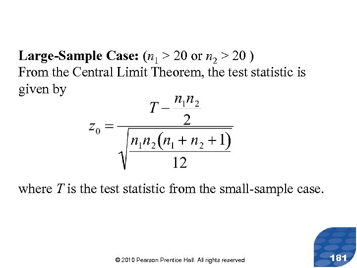 Large-Sample Case: (n 1 > 20 or n 2 > 20 ) From the Central Limit Theorem, the test statistic is given by where T is the test statistic from the small-sample case. © 2010 Pearson Prentice Hall. All rights reserved 181
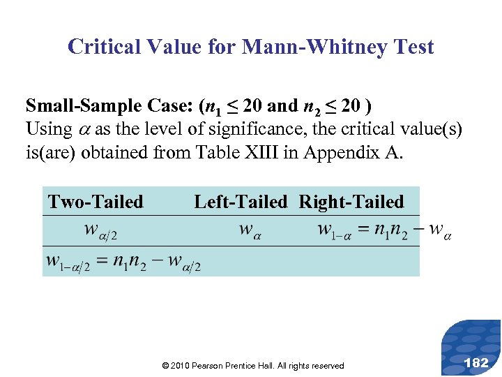 Critical Value for Mann-Whitney Test Small-Sample Case: (n 1 ≤ 20 and n 2 ≤ 20 ) Using as the level of significance, the critical value(s) is(are) obtained from Table XIII in Appendix A. Two-Tailed Left-Tailed Right-Tailed © 2010 Pearson Prentice Hall. All rights reserved 182
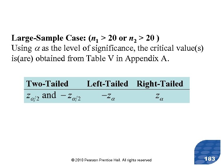 Large-Sample Case: (n 1 > 20 or n 2 > 20 ) Using as the level of significance, the critical value(s) is(are) obtained from Table V in Appendix A. Two-Tailed Left-Tailed Right-Tailed © 2010 Pearson Prentice Hall. All rights reserved 183
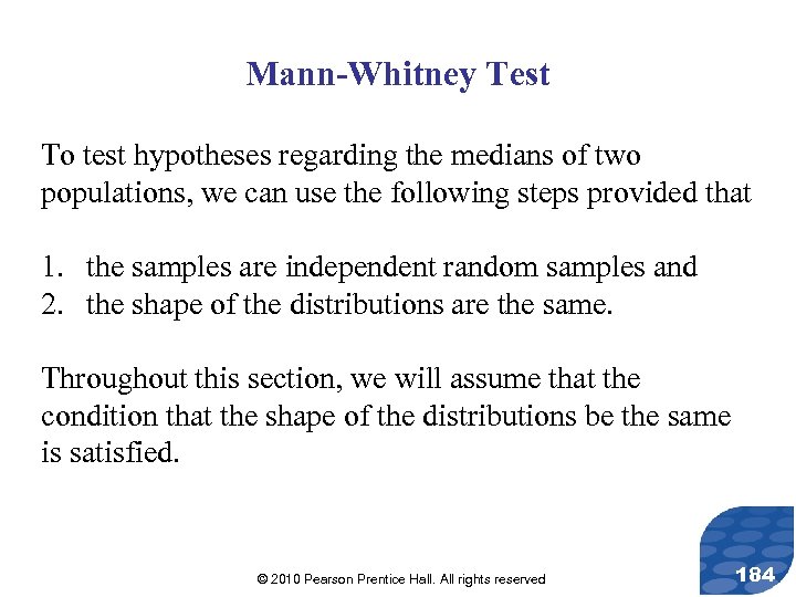 Mann-Whitney Test To test hypotheses regarding the medians of two populations, we can use the following steps provided that 1. the samples are independent random samples and 2. the shape of the distributions are the same. Throughout this section, we will assume that the condition that the shape of the distributions be the same is satisfied. © 2010 Pearson Prentice Hall. All rights reserved 184
 Step 1: Draw a side-by-side boxplot to compare the sample data from the two populations. This helps to visualize the difference in the medians. © 2010 Pearson Prentice Hall. All rights reserved 185
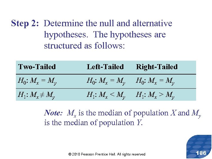 Step 2: Determine the null and alternative hypotheses. The hypotheses are structured as follows: Two-Tailed Left-Tailed Right-Tailed H 0: Mx = My H 1: Mx ≠ My H 1: Mx < My H 1: Mx > My Note: Mx is the median of population X and My is the median of population Y. © 2010 Pearson Prentice Hall. All rights reserved 186
 Step 3: Rank all sample observations from smallest to largest. Handle ties by finding the mean of the ranks for tied values. Find the sum of the ranks for the sample from population X. © 2010 Pearson Prentice Hall. All rights reserved 187
 Step 4: Choose a level of significance, , to match the seriousness of making a Type I error. The level of significance is used to determine the critical value. The critical value is found from Table XIII for small samples (n 1 ≤ 20 and n 2 ≤ 20) and from Table V for large samples (n 1 > 20 or n 2 > 20). © 2010 Pearson Prentice Hall. All rights reserved 188
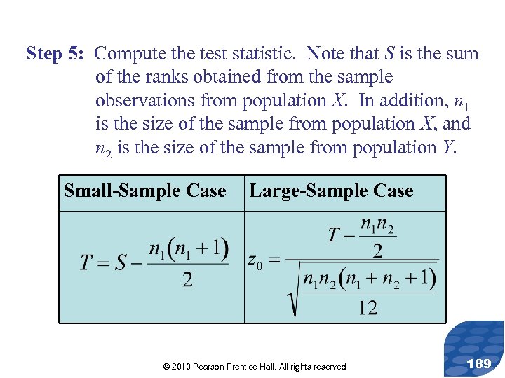 Step 5: Compute the test statistic. Note that S is the sum of the ranks obtained from the sample observations from population X. In addition, n 1 is the size of the sample from population X, and n 2 is the size of the sample from population Y. Small-Sample Case Large-Sample Case © 2010 Pearson Prentice Hall. All rights reserved 189
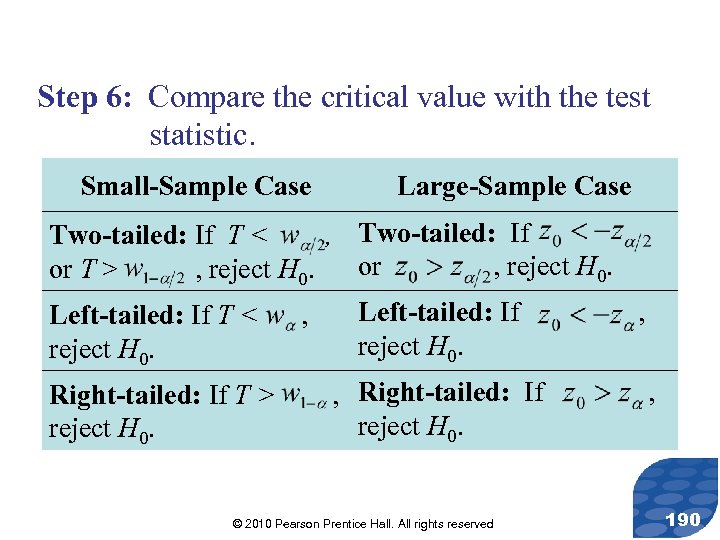 Step 6: Compare the critical value with the test statistic. Small-Sample Case Large-Sample Case Two-tailed: If T < , Two-tailed: If or , reject H 0. or T > , reject H 0. Left-tailed: If T < reject H 0. Right-tailed: If T > reject H 0. , Left-tailed: If reject H 0. , Right-tailed: If reject H 0. © 2010 Pearson Prentice Hall. All rights reserved , , 190
 Step 7: State the conclusion. © 2010 Pearson Prentice Hall. All rights reserved 191
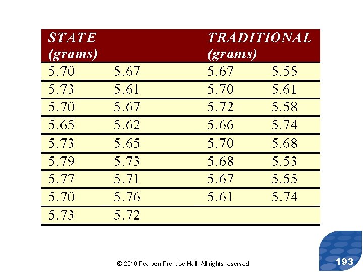
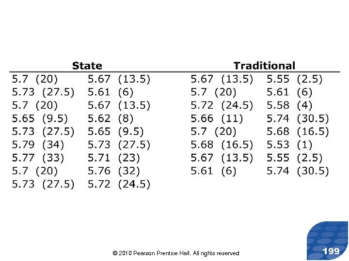
 Parallel Example 1: Mann-Whitney Test (Small-Sample Case) A researcher wanted to know whether “state” quarters had a weight that is more than “traditional” quarters. He randomly selected 18 “state” quarters and 16 “traditional” quarters, weighed each of them and obtained the following data. © 2010 Pearson Prentice Hall. All rights reserved 192
 © 2010 Pearson Prentice Hall. All rights reserved 193
 Parallel Example 1: Mann-Whitney Test (Small-Sample Case) Test the claim that state quarters have a higher median weight than traditional quarters at the =0. 05 level of significance. © 2010 Pearson Prentice Hall. All rights reserved 194
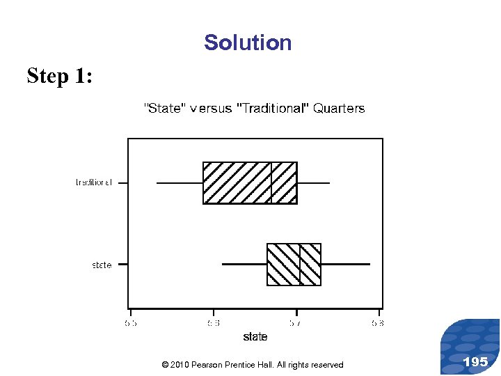 Solution Step 1: © 2010 Pearson Prentice Hall. All rights reserved 195
 Solution Step 1: Based on the boxplots, the median weight for the state quarters is higher. We want to estimate whether this difference is due to differences in the population medians or to sampling error. © 2010 Pearson Prentice Hall. All rights reserved 196
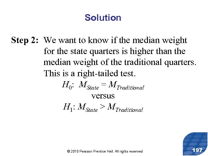 Solution Step 2: We want to know if the median weight for the state quarters is higher than the median weight of the traditional quarters. This is a right-tailed test. H 0: MState = MTraditional versus H 1: MState > MTraditional © 2010 Pearson Prentice Hall. All rights reserved 197
 Solution Step 3: In order to calculate the test statistic, we combine the two data sets into one data set and arrange the data in ascending order. Ranks are shown on the following slide. © 2010 Pearson Prentice Hall. All rights reserved 198
 © 2010 Pearson Prentice Hall. All rights reserved 199
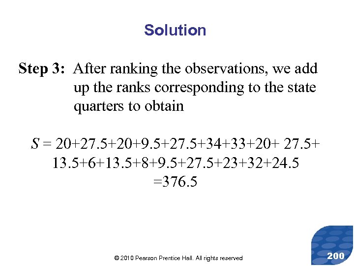 Solution Step 3: After ranking the observations, we add up the ranks corresponding to the state quarters to obtain S = 20+27. 5+20+9. 5+27. 5+34+33+20+ 27. 5+ 13. 5+6+13. 5+8+9. 5+27. 5+23+32+24. 5 =376. 5 © 2010 Pearson Prentice Hall. All rights reserved 200
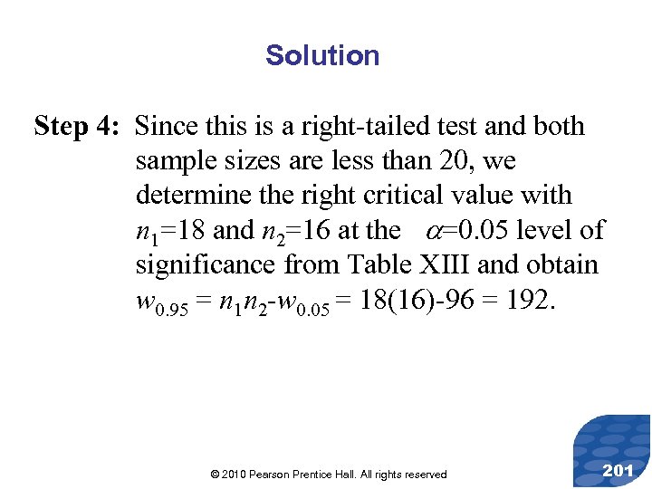 Solution Step 4: Since this is a right-tailed test and both sample sizes are less than 20, we determine the right critical value with n 1=18 and n 2=16 at the =0. 05 level of significance from Table XIII and obtain w 0. 95 = n 1 n 2 -w 0. 05 = 18(16)-96 = 192. © 2010 Pearson Prentice Hall. All rights reserved 201
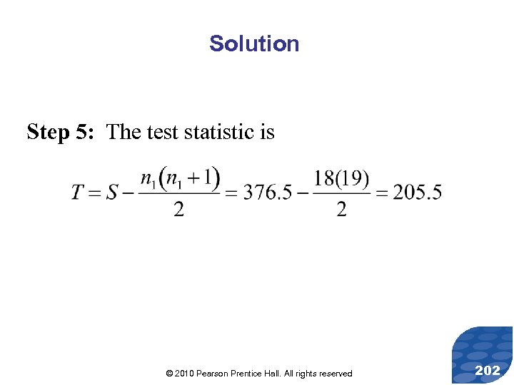 Solution Step 5: The test statistic is © 2010 Pearson Prentice Hall. All rights reserved 202
 Solution Step 6: Since the test statistic is greater than the critical value (205. 5 > 192), we reject the null hypothesis. Step 7: There is sufficient evidence at the = 0. 05 level of significance to conclude that the median weight of “state” quarters is greater than that of “traditional” quarters. © 2010 Pearson Prentice Hall. All rights reserved 203
 Section 15. 6 Spearman’s Rank. Correlation Test © 2010 Pearson Prentice Hall. All rights reserved
 Objective 1. Perform Spearman’s rank-correlation test © 2010 Pearson Prentice Hall. All rights reserved 205
 The Spearman’s rank-correlation test is a nonparametric procedure that is used to test hypotheses regarding the association between two variables. © 2010 Pearson Prentice Hall. All rights reserved 206
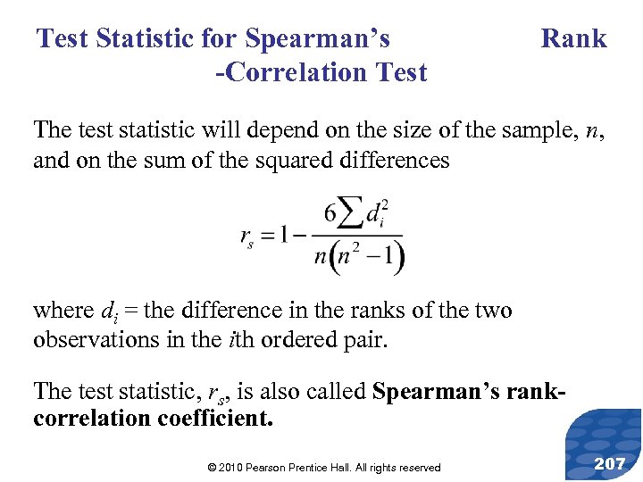 Test Statistic for Spearman’s -Correlation Test Rank The test statistic will depend on the size of the sample, n, and on the sum of the squared differences where di = the difference in the ranks of the two observations in the ith ordered pair. The test statistic, rs, is also called Spearman’s rankcorrelation coefficient. © 2010 Pearson Prentice Hall. All rights reserved 207
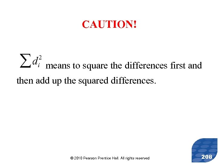 CAUTION! means to square the differences first and then add up the squared differences. © 2010 Pearson Prentice Hall. All rights reserved 208
 Critical Value for Spearman’s -Correlation Test Rank Using as the level of significance, the critical value(s) is(are) obtained from Table XIV in Appendix A. For a two-tailed test, be sure to divide the level of significance, , by 2. © 2010 Pearson Prentice Hall. All rights reserved 209
 Spearman’s Rank-Correlation Test To test hypotheses regarding the association between two variables X and Y, we can use the following steps, provided that 1. the data are a random sample of n ordered pairs and 2. each pair of observations is two measurements taken on the same individual. Notice that there is no requirement about the form of the distribution of the data. © 2010 Pearson Prentice Hall. All rights reserved 210
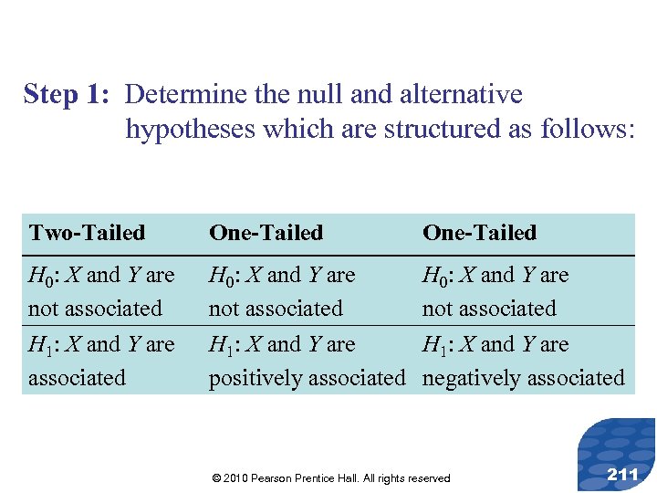 Step 1: Determine the null and alternative hypotheses which are structured as follows: Two-Tailed One-Tailed H 0: X and Y are not associated H 1: X and Y are associated H 0: X and Y are not associated H 1: X and Y are positively associated H 0: X and Y are not associated H 1: X and Y are negatively associated © 2010 Pearson Prentice Hall. All rights reserved 211
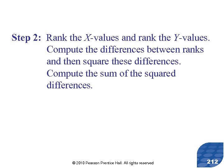 Step 2: Rank the X-values and rank the Y-values. Compute the differences between ranks and then square these differences. Compute the sum of the squared differences. © 2010 Pearson Prentice Hall. All rights reserved 212
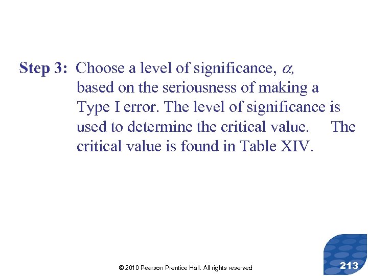 Step 3: Choose a level of significance, , based on the seriousness of making a Type I error. The level of significance is used to determine the critical value. The critical value is found in Table XIV. © 2010 Pearson Prentice Hall. All rights reserved 213
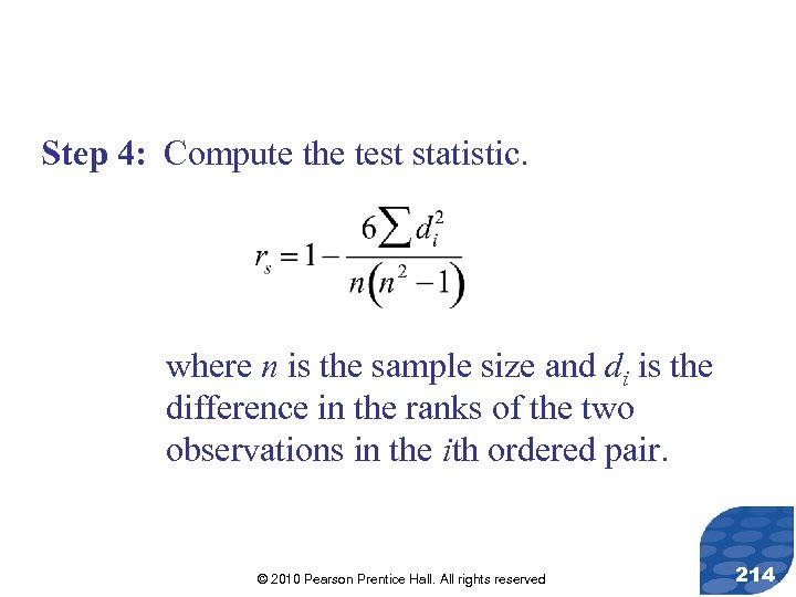 Step 4: Compute the test statistic. where n is the sample size and di is the difference in the ranks of the two observations in the ith ordered pair. © 2010 Pearson Prentice Hall. All rights reserved 214
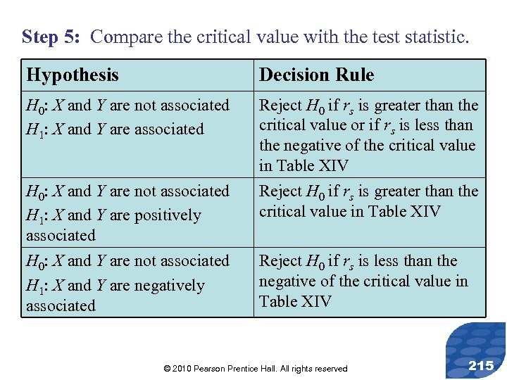 Step 5: Compare the critical value with the test statistic. Hypothesis Decision Rule H 0: X and Y are not associated H 1: X and Y are associated Reject H 0 if rs is greater than the critical value or if rs is less than the negative of the critical value in Table XIV H 0: X and Y are not associated H 1: X and Y are positively associated H 0: X and Y are not associated H 1: X and Y are negatively associated Reject H 0 if rs is greater than the critical value in Table XIV Reject H 0 if rs is less than the negative of the critical value in Table XIV © 2010 Pearson Prentice Hall. All rights reserved 215
 Step 6: State the conclusion. © 2010 Pearson Prentice Hall. All rights reserved 216
 Parallel Example 1: Spearman’s Rank-Correlation Test Is the price of a sport’s car associated with its performance? The following data represent the ranks of the price and performance of 8 sport’s cars. Using Spearman’s Rank Correlation, determine if the two variables are associated at the = 0. 05 level of significance. © 2010 Pearson Prentice Hall. All rights reserved 217
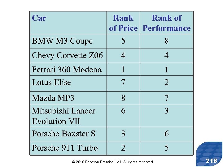 Car BMW M 3 Coupe Rank of of Price Performance 5 8 Chevy Corvette Z 06 4 4 Ferrari 360 Modena Lotus Elise 1 7 1 2 Mazda MP 3 Mitsubishi Lancer Evolution VII Porsche Boxster S 8 6 7 3 3 6 Porsche 911 Turbo 2 5 © 2010 Pearson Prentice Hall. All rights reserved 218
 Solution Step 1: We are looking for evidence that price and performance of sport’s cars are associated. Let X represent the price of the sport’s car and Y represent performance. The null and alternative hypotheses are as follows: H 0: X and Y are not associated H 1: X and Y are associated © 2010 Pearson Prentice Hall. All rights reserved 219
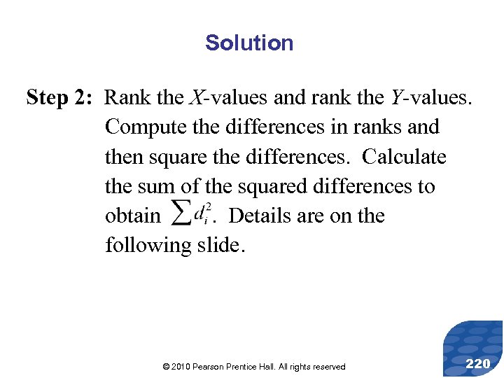 Solution Step 2: Rank the X-values and rank the Y-values. Compute the differences in ranks and then square the differences. Calculate the sum of the squared differences to obtain. Details are on the following slide. © 2010 Pearson Prentice Hall. All rights reserved 220
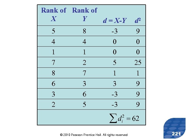 Rank of X Y d = X-Y 5 8 -3 4 4 0 1 1 0 7 2 5 8 7 1 6 3 3 3 6 -3 2 5 -3 © 2010 Pearson Prentice Hall. All rights reserved d 2 9 0 0 25 1 9 9 9 221
 Solution Step 3: This is a two-tailed test with n=8 and = 0. 05. From Table XIV we determine the critical value to be 0. 738. © 2010 Pearson Prentice Hall. All rights reserved 222
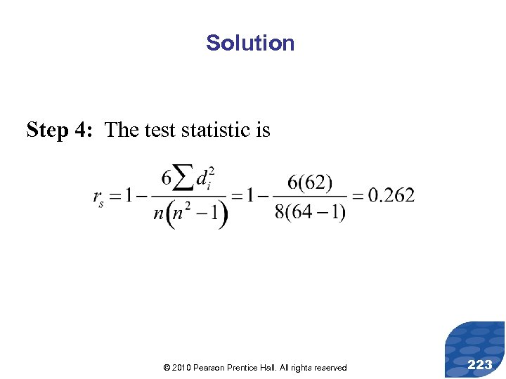 Solution Step 4: The test statistic is © 2010 Pearson Prentice Hall. All rights reserved 223
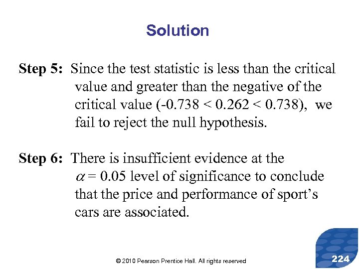 Solution Step 5: Since the test statistic is less than the critical value and greater than the negative of the critical value (-0. 738 < 0. 262 < 0. 738), we fail to reject the null hypothesis. Step 6: There is insufficient evidence at the = 0. 05 level of significance to conclude that the price and performance of sport’s cars are associated. © 2010 Pearson Prentice Hall. All rights reserved 224
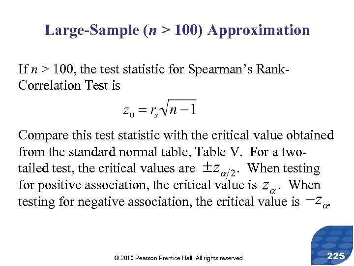 Large-Sample (n > 100) Approximation If n > 100, the test statistic for Spearman’s Rank. Correlation Test is Compare this test statistic with the critical value obtained from the standard normal table, Table V. For a twotailed test, the critical values are. When testing for positive association, the critical value is. When testing for negative association, the critical value is. © 2010 Pearson Prentice Hall. All rights reserved 225
 Section 15. 7 Kruskal-Wallis Test © 2010 Pearson Prentice Hall. All rights reserved
 Objective 1. Test a hypothesis using the Kruskal-Wallis test © 2010 Pearson Prentice Hall. All rights reserved 227
 The Kruskal-Wallis Test is a nonparametric procedure that is used to test whether k independent samples come from populations with the same distribution. © 2010 Pearson Prentice Hall. All rights reserved 228
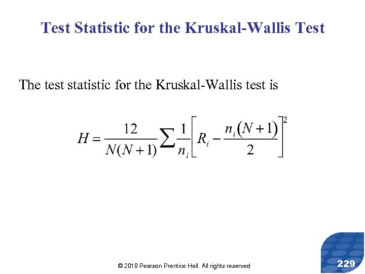 Test Statistic for the Kruskal-Wallis Test The test statistic for the Kruskal-Wallis test is © 2010 Pearson Prentice Hall. All rights reserved 229
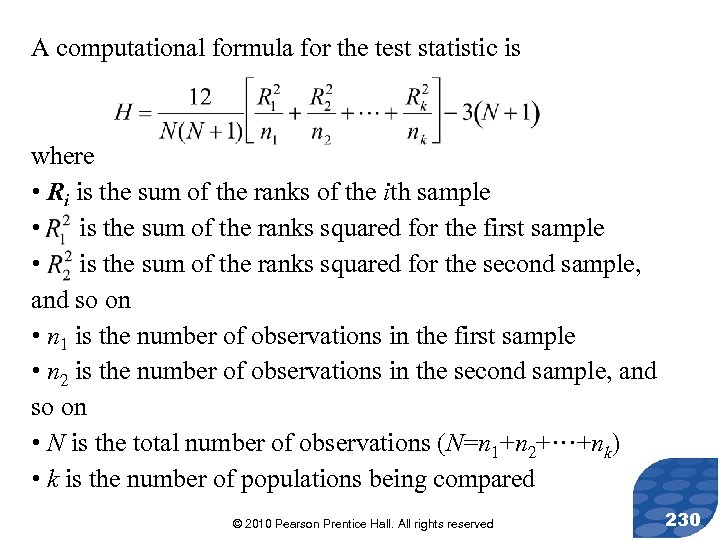 A computational formula for the test statistic is where • Ri is the sum of the ranks of the ith sample • is the sum of the ranks squared for the first sample • is the sum of the ranks squared for the second sample, and so on • n 1 is the number of observations in the first sample • n 2 is the number of observations in the second sample, and so on • N is the total number of observations (N=n 1+n 2+···+nk) • k is the number of populations being compared © 2010 Pearson Prentice Hall. All rights reserved 230
 Critical Value for Kruskal-Wallis Test Small-Sample Case When three populations are being compared and when the sample size from each population is 5 or less, the critical value is obtained from Table XV in Appendix A. Large-Sample Case When four or more populations are being compared or the sample size from one population is more than 5, the critical value is with k-1 degrees of freedom, where k is the number of populations and is the level of significance. © 2010 Pearson Prentice Hall. All rights reserved 231
 Kruskal-Wallis Test To test hypotheses regarding the distribution of three or more populations, we can use the following steps, provided that two requirements are satisfied: 1. The samples are independent random samples 2. The data can be ranked Step 1: Draw side-by-side boxplots to compare the sample data from the populations. Doing so helps to visualize the differences, if any, between the medians. © 2010 Pearson Prentice Hall. All rights reserved 232
 Step 2: State the null and alternative hypotheses, which are structured as follows: H 0: the distributions of the populations are the same H 1: the distributions of the populations are not the same Step 3: Rank all sample observations from smallest to largest. Handle ties by finding the mean of the ranks for tied values. Find the sum of the ranks for each sample. © 2010 Pearson Prentice Hall. All rights reserved 233
 Step 4: Choose a level of significance, , to match the seriousness of making a Type I error. The level of significance is used to determine the critical value. The critical value is found from Table XV for small samples. The critical value is with k-1 degrees of freedom (found in Table VII) for large samples. © 2010 Pearson Prentice Hall. All rights reserved 234
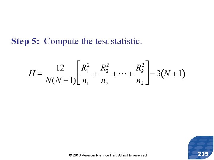 Step 5: Compute the test statistic. © 2010 Pearson Prentice Hall. All rights reserved 235
 Step 6: Compare the critical value to the test statistic. We reject the null hypothesis if the test statistic is greater than the critical value. © 2010 Pearson Prentice Hall. All rights reserved 236
 Step 7: State the conclusion. © 2010 Pearson Prentice Hall. All rights reserved 237
 Parallel Example 1: Kruskal-Wallis Test The following data represent the weight (in grams) of pennies minted at the Denver mint in 1990, 1995, and 2000. Test the claim that the distribution of penny weights differs for the three years at the = 0. 05 level of significance. © 2010 Pearson Prentice Hall. All rights reserved 238
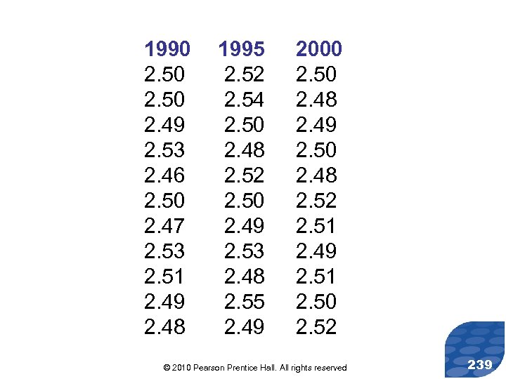 1990 2. 50 2. 49 2. 53 2. 46 2. 50 2. 47 2. 53 2. 51 2. 49 2. 48 1995 2. 52 2. 54 2. 50 2. 48 2. 52 2. 50 2. 49 2. 53 2. 48 2. 55 2. 49 2000 2. 50 2. 48 2. 49 2. 50 2. 48 2. 52 2. 51 2. 49 2. 51 2. 50 2. 52 © 2010 Pearson Prentice Hall. All rights reserved 239
 Solution The samples are independent random samples that can be ranked. Therefore, the conditions for the Kruskal-Wallis test are met. © 2010 Pearson Prentice Hall. All rights reserved 240
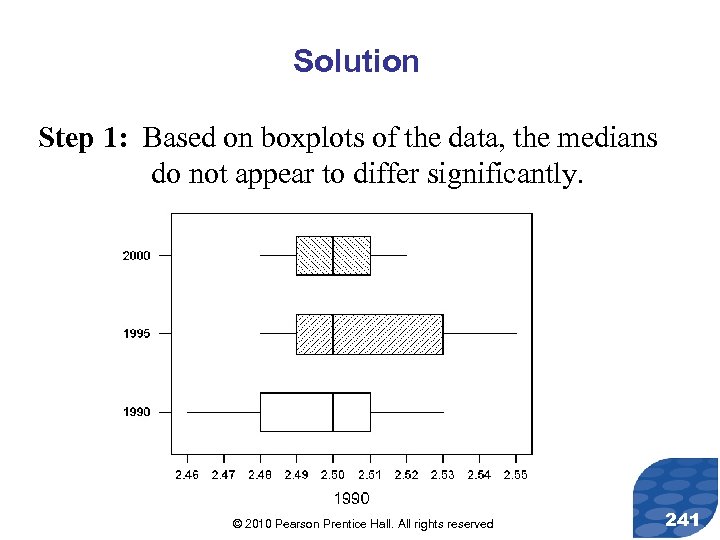 Solution Step 1: Based on boxplots of the data, the medians do not appear to differ significantly. © 2010 Pearson Prentice Hall. All rights reserved 241
 Solution Step 2: We are interested in determining whether the distribution of penny weights differs for the three years. The null and alternative hypotheses are as follows: H 0: the distribution of penny weights are the same for the three years H 1: the distribution of penny weights are not the same for the three years © 2010 Pearson Prentice Hall. All rights reserved 242
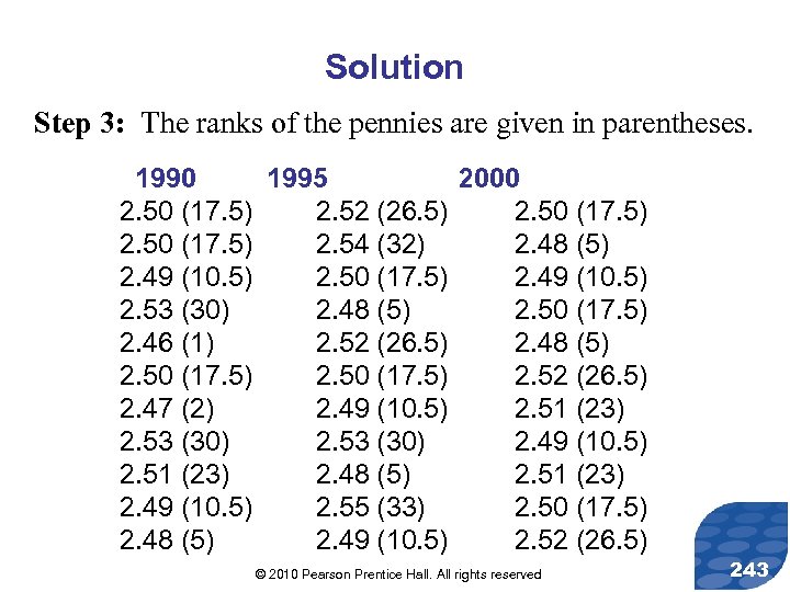 Solution Step 3: The ranks of the pennies are given in parentheses. 1990 1995 2000 2. 50 (17. 5) 2. 52 (26. 5) 2. 50 (17. 5) 2. 54 (32) 2. 48 (5) 2. 49 (10. 5) 2. 50 (17. 5) 2. 49 (10. 5) 2. 53 (30) 2. 48 (5) 2. 50 (17. 5) 2. 46 (1) 2. 52 (26. 5) 2. 48 (5) 2. 50 (17. 5) 2. 52 (26. 5) 2. 47 (2) 2. 49 (10. 5) 2. 51 (23) 2. 53 (30) 2. 49 (10. 5) 2. 51 (23) 2. 48 (5) 2. 51 (23) 2. 49 (10. 5) 2. 55 (33) 2. 50 (17. 5) 2. 48 (5) 2. 49 (10. 5) 2. 52 (26. 5) © 2010 Pearson Prentice Hall. All rights reserved 243
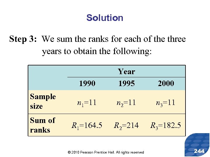 Solution Step 3: We sum the ranks for each of the three years to obtain the following: 1990 Year 1995 2000 Sample size n 1=11 n 2=11 n 3=11 Sum of ranks R 1=164. 5 R 2=214 R 3=182. 5 © 2010 Pearson Prentice Hall. All rights reserved 244
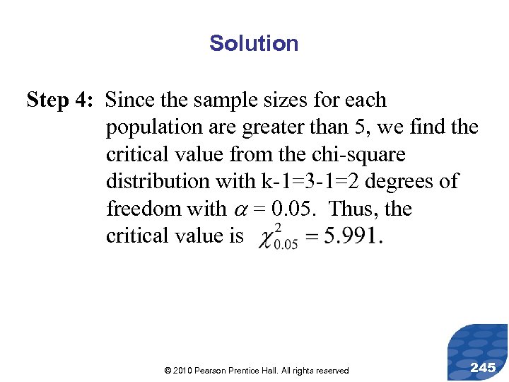 Solution Step 4: Since the sample sizes for each population are greater than 5, we find the critical value from the chi-square distribution with k-1=3 -1=2 degrees of freedom with = 0. 05. Thus, the critical value is © 2010 Pearson Prentice Hall. All rights reserved 245
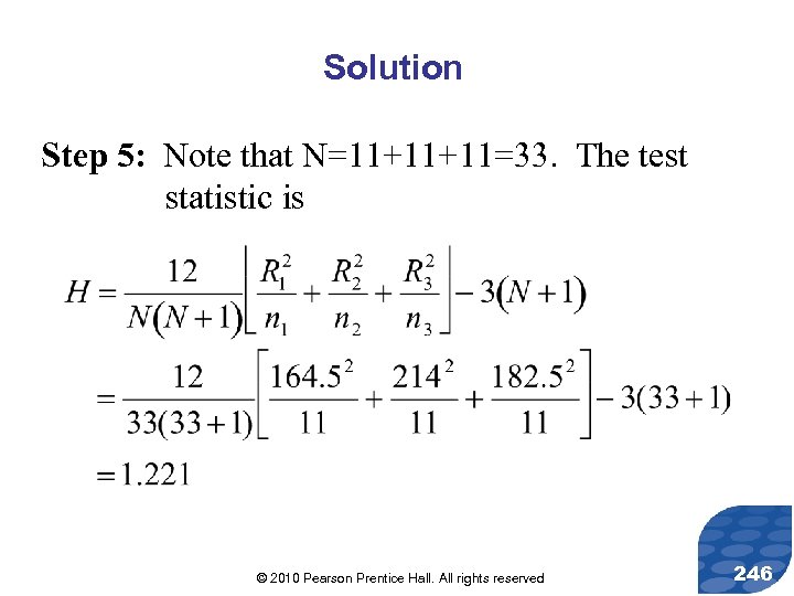 Solution Step 5: Note that N=11+11+11=33. The test statistic is © 2010 Pearson Prentice Hall. All rights reserved 246
 Solution Step 6: Since the test statistic is less than the critical value, we fail to reject the null hypothesis. Step 7: There is insufficient evidence at the = 0. 05 level of significance to conclude that the distribution of penny weights differs for the years 1990, 1995 and 2000. © 2010 Pearson Prentice Hall. All rights reserved 247


