455315e2f656e9cfeac4c0353270d64d.ppt
- Количество слайдов: 40
 Chapter 14 Oligopoly and Monopolistic Competition Anyone can win unless there happens to be a second entry. George Ade
 Chapter 14 Outline Challenge: Government Aircraft Subsidies 14. 1 Market Structures 14. 2 Cartels 14. 3 Cournot Oligopoly Model 14. 4 Stackelberg Oligopoly Model 14. 5 Bertrand Oligopoly Model 14. 6 Monopolistic Competition Challenge Solution Copyright © 2014 Pearson Education, Inc. All rights reserved. 14 -2
 Challenge: Government Aircraft Subsidies • Background: • Governments consistently intervene in aircraft manufacturing markets. • France, Germany, Spain, and the United Kingdom jointly own and heavily subsidize Airbus • Questions: • If only one government subsidizes its firm, what is the effect on price and quantity in the aircraft manufacturing market? (See Solved Problem 14. 3) • What happens if both governments subsidize their firms? (See Challenge Solution) Copyright © 2014 Pearson Education, Inc. All rights reserved. 14 -3
 14. 1 Market Structures • Markets differ according to • the number of firms in the market • the ease with which firms may enter and leave the market • the ability of firms to differentiate their products from rivals’ • Oligopoly is a market structure in which a small group of firms each influence price and enjoy substantial barriers to entry. • Example: video game producers (Nintendo, Microsoft, Sony) • Monopolistic competition is a market structure in which firms have market power but no additional firm can enter and earn a positive profit. • Example: laundry detergent Copyright © 2014 Pearson Education, Inc. All rights reserved. 14 -4
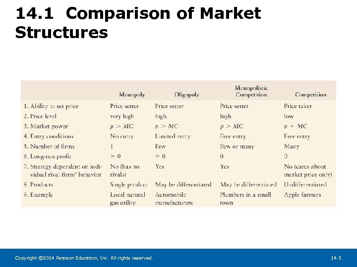 14. 1 Comparison of Market Structures Copyright © 2014 Pearson Education, Inc. All rights reserved. 14 -5
 14. 2 Cartels • Oligopolistic firms have an incentive to collude, coordinate setting their prices or quantities, so as to increase their profits. • Collusion is illegal in most developed countries. • A cartel, a group of firms that collude, is a special case of oligopoly in which the firms behave like a monopoly. • Because firms can make even more money by cheating on the cartel agreement, collusion is not always successful. Copyright © 2014 Pearson Education, Inc. All rights reserved. 14 -6
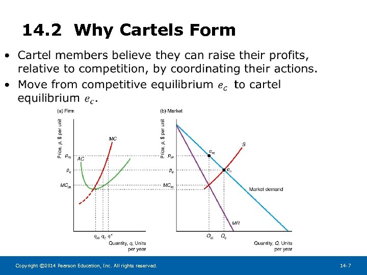 14. 2 Why Cartels Form • Copyright © 2014 Pearson Education, Inc. All rights reserved. 14 -7
 14. 2 Laws Against Cartels • Previously called trusts in the U. S. and common in oil, railroad, sugar, and tobacco industries • Sherman Antitrust Act (1890) and Federal Trade Commission Act (1914) • Prohibit firms from explicitly agreeing to take actions that reduce competition • Jointly setting price strictly prohibited • Antitrust laws reduce probability that cartels form • OPEC, most famous cartel, formed in 1960 and is not illegal among participating countries. Copyright © 2014 Pearson Education, Inc. All rights reserved. 14 -8
 14. 2 Cartels • Why Cartels Fail • Cartels fail if noncartel members can supply consumers with large quantities of goods. • Each member of a cartel has an incentive to cheat on the cartel agreement. • Maintaining Cartels • Detection of cheating and enforcement • Government support • Barriers to entry (fewer firms makes cheating easier to detect) • Mergers Copyright © 2014 Pearson Education, Inc. All rights reserved. 14 -9
 14. 3 Cournot Oligopoly Model • The Cournot model explains how oligopoly firms behave if they simultaneously choose how much they produce. • Four main assumptions: 1. There are two firms and no others can enter the market 2. The firms have identical costs 3. The firms sell identical products 4. The firms set their quantities simultaneously • Example: Airline market Copyright © 2014 Pearson Education, Inc. All rights reserved. 14 -10
 14. 3 Cournot Model of an Airline Market • Recall the interaction between American Airlines and United Airlines from Chapter 13. • In normal-form game, we assumed airlines chose between two output levels. • We generalize that example; firms choose any output level. • The Cournot equilibrium (or Nash-Cournot equilibrium) in this model is a set of quantities chosen by firms such that, holding quantities of other firms constant, no firm can obtain higher profit by choosing a different quantity. Copyright © 2014 Pearson Education, Inc. All rights reserved. 14 -11
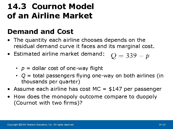 14. 3 Cournot Model of an Airline Market Demand Cost • The quantity each airline chooses depends on the residual demand curve it faces and its marginal cost. • Estimated airline market demand: • p = dollar cost of one-way flight • Q = total passengers flying one-way on both airlines (in thousands per quarter) • Assume each airline has cost MC = $147 per passenger • How does the monopoly outcome compare to duopoly (Cournot with two firms)? Copyright © 2014 Pearson Education, Inc. All rights reserved. 14 -12
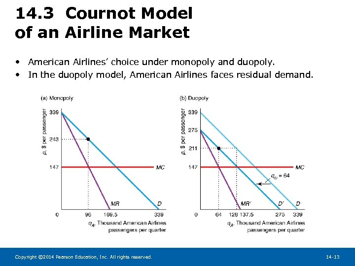 14. 3 Cournot Model of an Airline Market • American Airlines’ choice under monopoly and duopoly. • In the duopoly model, American Airlines faces residual demand. Copyright © 2014 Pearson Education, Inc. All rights reserved. 14 -13
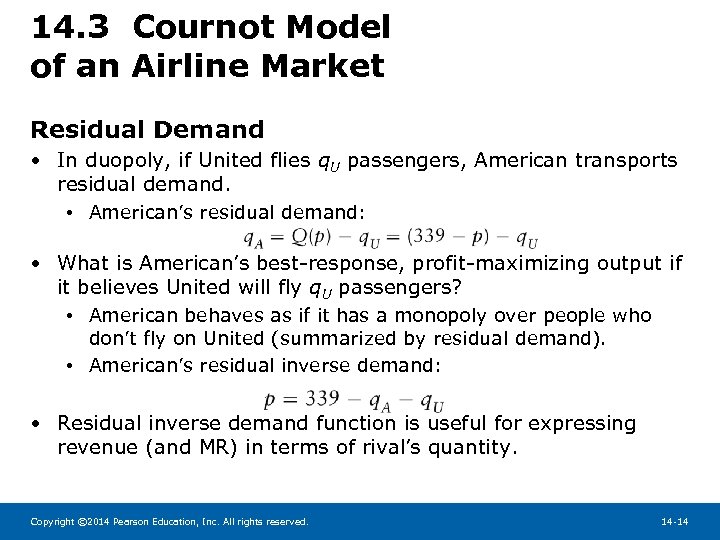 14. 3 Cournot Model of an Airline Market Residual Demand • In duopoly, if United flies q. U passengers, American transports residual demand. • American’s residual demand: • What is American’s best-response, profit-maximizing output if it believes United will fly q. U passengers? • American behaves as if it has a monopoly over people who don’t fly on United (summarized by residual demand). • American’s residual inverse demand: • Residual inverse demand function is useful for expressing revenue (and MR) in terms of rival’s quantity. Copyright © 2014 Pearson Education, Inc. All rights reserved. 14 -14
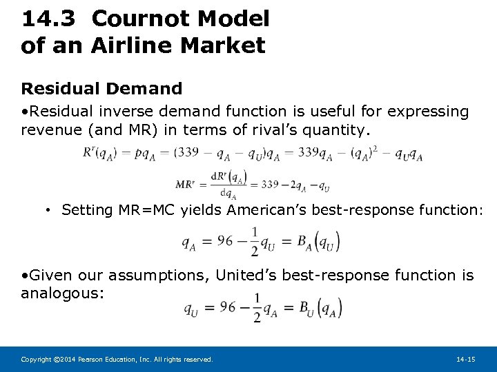 14. 3 Cournot Model of an Airline Market Residual Demand • Residual inverse demand function is useful for expressing revenue (and MR) in terms of rival’s quantity. • Setting MR=MC yields American’s best-response function: • Given our assumptions, United’s best-response function is analogous: Copyright © 2014 Pearson Education, Inc. All rights reserved. 14 -15
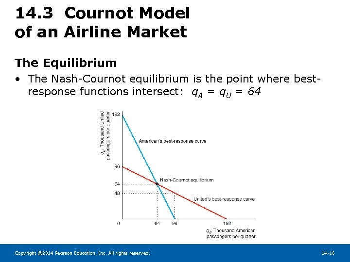 14. 3 Cournot Model of an Airline Market The Equilibrium • The Nash-Cournot equilibrium is the point where bestresponse functions intersect: q. A = q. U = 64 Copyright © 2014 Pearson Education, Inc. All rights reserved. 14 -16
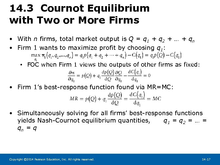 14. 3 Cournot Equilibrium with Two or More Firms • With n firms, total market output is Q = q 1 + q 2 + … + qn • Firm 1 wants to maximize profit by choosing q 1: • FOC when Firm 1 views the outputs of other firms as fixed: • Firm 1’s best-response function found via MR=MC: • Simultaneously solving for all firms’ best-response functions yields Nash-Cournot equilibrium quantities, q 1 = q 2 = … = qn = q Copyright © 2014 Pearson Education, Inc. All rights reserved. 14 -17
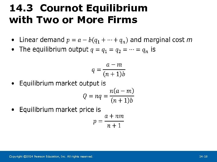 14. 3 Cournot Equilibrium with Two or More Firms • Copyright © 2014 Pearson Education, Inc. All rights reserved. 14 -18
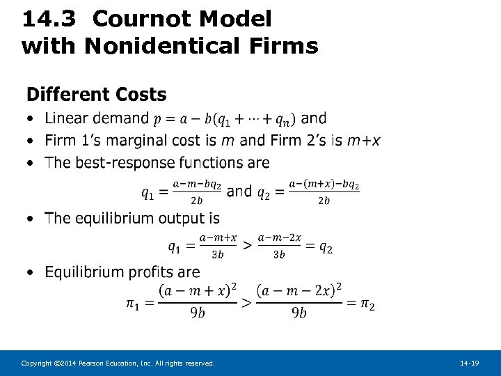 14. 3 Cournot Model with Nonidentical Firms • Copyright © 2014 Pearson Education, Inc. All rights reserved. 14 -19
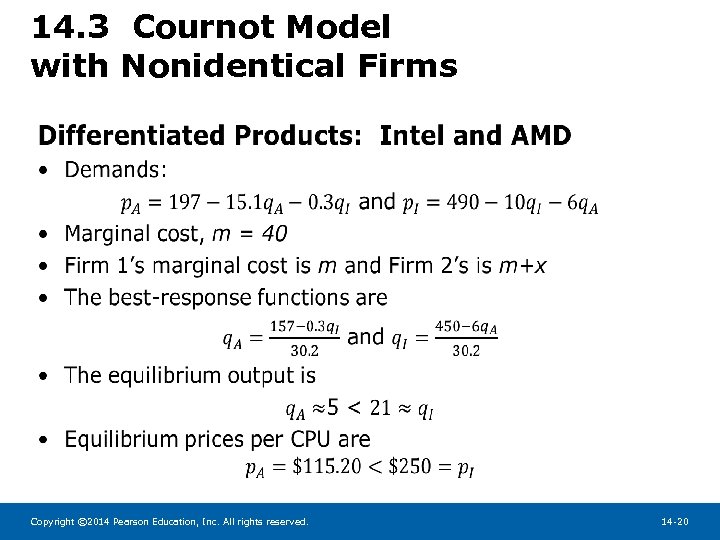 14. 3 Cournot Model with Nonidentical Firms • Copyright © 2014 Pearson Education, Inc. All rights reserved. 14 -20
 14. 4 Stackelberg Oligopoly Model • Suppose that one of the firms in our previous example was the leader and set its output before its rival, the follower. • Does the firm that acts first have an advantage? • How does this model’s outcome differ from the Cournot oligopoly model? • The Stackelberg model of oligopoly addresses these questions. • Note that once the leader sets its output, the rival firm will use its Cournot best-response curve to set its output. Copyright © 2014 Pearson Education, Inc. All rights reserved. 14 -21
 14. 4 Stackelberg Oligopoly Model • General linear inverse demand function: p = a – b. Q • Two firms have identical marginal costs, m • Firm 1 (American Airlines) is the Stackelberg leader and chooses output first • Firm 2 (United Airlines) is the follower and chooses output using best-response function • The Stackelberg leader knows the follower will use its best-response function and so the leader views the residual demand in the market as its demand. Copyright © 2014 Pearson Education, Inc. All rights reserved. 14 -22
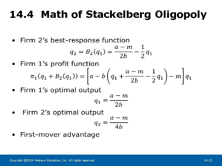 14. 4 Math of Stackelberg Oligopoly • Copyright © 2014 Pearson Education, Inc. All rights reserved. 14 -23
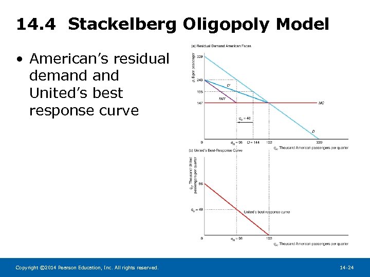 14. 4 Stackelberg Oligopoly Model • American’s residual demand United’s best response curve Copyright © 2014 Pearson Education, Inc. All rights reserved. 14 -24
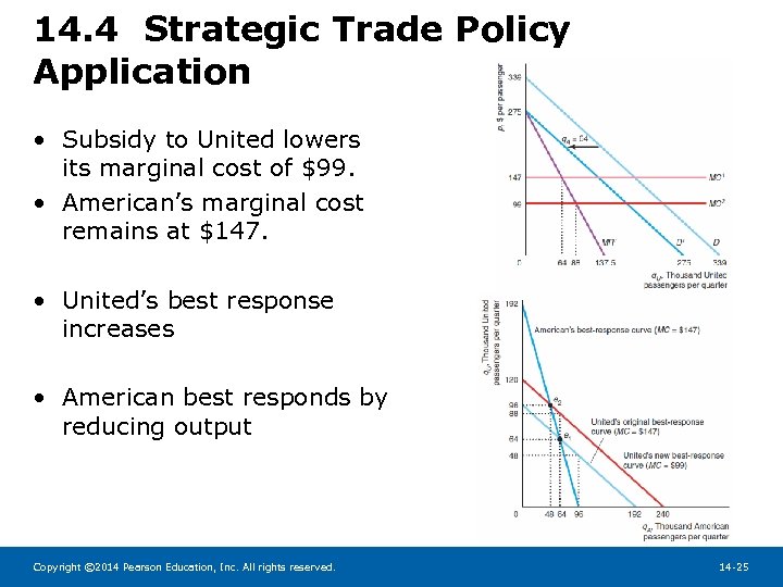 14. 4 Strategic Trade Policy Application • Subsidy to United lowers its marginal cost of $99. • American’s marginal cost remains at $147. • United’s best response increases • American best responds by reducing output Copyright © 2014 Pearson Education, Inc. All rights reserved. 14 -25
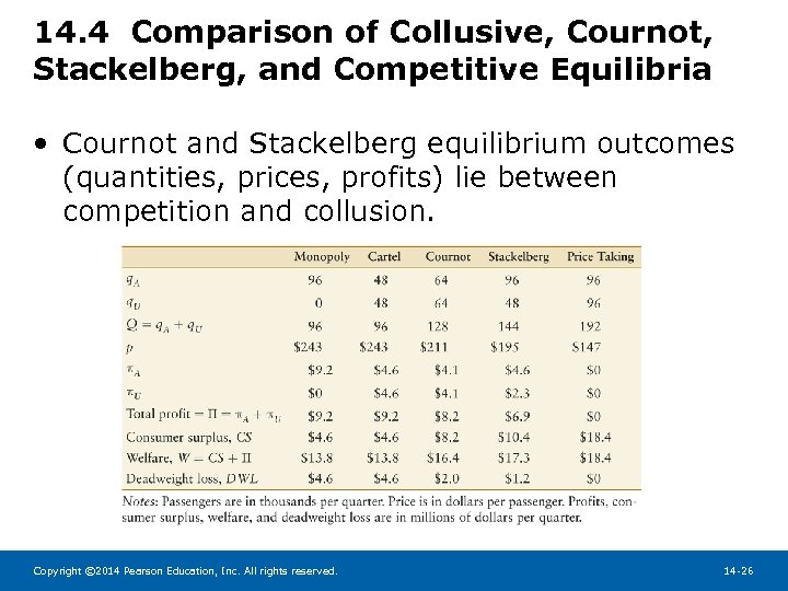 14. 4 Comparison of Collusive, Cournot, Stackelberg, and Competitive Equilibria • Cournot and Stackelberg equilibrium outcomes (quantities, prices, profits) lie between competition and collusion. Copyright © 2014 Pearson Education, Inc. All rights reserved. 14 -26
 14. 4 Comparison of Collusive, Cournot, Stackelberg, and Competitive Equilibria Copyright © 2014 Pearson Education, Inc. All rights reserved. 14 -27
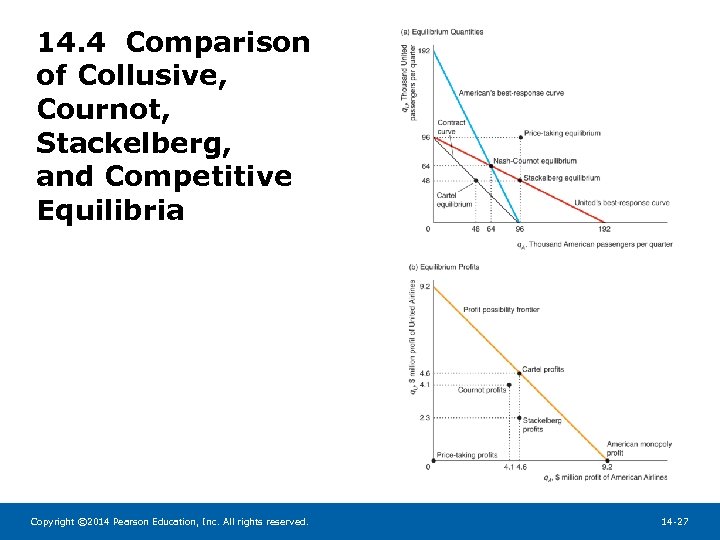
 14. 4 Comparison of Collusive, Cournot, Stackelberg, and Competitive Equilibria • These four equilibrium outcomes can also be compared graphically. • Collusive output combinations are summarized on a “Contract curve. ” • Colluding firms could write a contract in which they agree to produce at any point along this curve. • Best-response curves are also depicted in order to show Cournot and Stackelberg equilibria. • Differences in quantities and profits are summarized graphically next. Copyright © 2014 Pearson Education, Inc. All rights reserved. 14 -28
 14. 5 Bertrand Oligopoly Model • What if, instead of setting quantities, firms set prices and allowed consumers to decide how much to buy? • A Bertrand equilibrium (or Nash-Bertrand equilibrium) is a set of prices such that no firm can obtain a higher profit by choosing a different price if the other firms continue to charge these prices. • The Bertrand equilibrium is different than a quantitysetting equilibrium in either the Cournot or Stackelberg models. Copyright © 2014 Pearson Education, Inc. All rights reserved. 14 -29
 14. 5 Bertrand Oligopoly Model • Assumptions of the model: • Firms have identical costs (and constant MC=$5) • Firms produce identical goods • Conditional on the price charged by Firm 2, p 2, Firm 1 wants to charge slightly less in order to attract customers. • If Firm 1 undercuts its rival’s price, Firm 1 captures entire market and earns all profit. • Thus, Firm 2 also has incentive to undercut Firm 1’s price. • Bertrand equilibrium price equals marginal cost (as in competition) because of incentive to undercut. Copyright © 2014 Pearson Education, Inc. All rights reserved. 14 -30
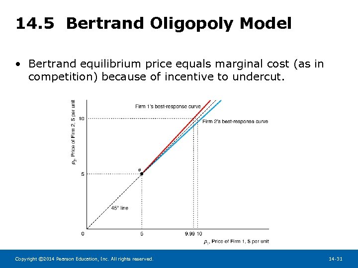 14. 5 Bertrand Oligopoly Model • Bertrand equilibrium price equals marginal cost (as in competition) because of incentive to undercut. Copyright © 2014 Pearson Education, Inc. All rights reserved. 14 -31
 14. 5 Nash-Bertrand Equilibrium with Differentiated Products • In many markets, firms produce differentiated goods. • Examples: automobiles, stereos, computers, toothpaste • Many economists believe that price-setting models are more plausible than quantity-setting models when goods are differentiated. • One firm can charge a higher price for its differentiated product without losing all its sales (e. g. Coke and Pepsi). • If we relax the “identical goods” assumption, the Bertrand model predicts that firms set prices above MC. Copyright © 2014 Pearson Education, Inc. All rights reserved. 14 -32
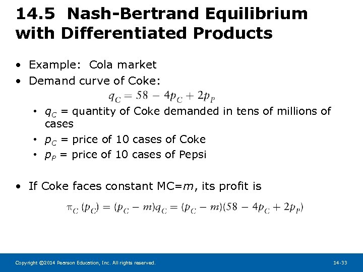 14. 5 Nash-Bertrand Equilibrium with Differentiated Products • Example: Cola market • Demand curve of Coke: • q. C = quantity of Coke demanded in tens of millions of cases • p. C = price of 10 cases of Coke • p. P = price of 10 cases of Pepsi • If Coke faces constant MC=m, its profit is Copyright © 2014 Pearson Education, Inc. All rights reserved. 14 -33
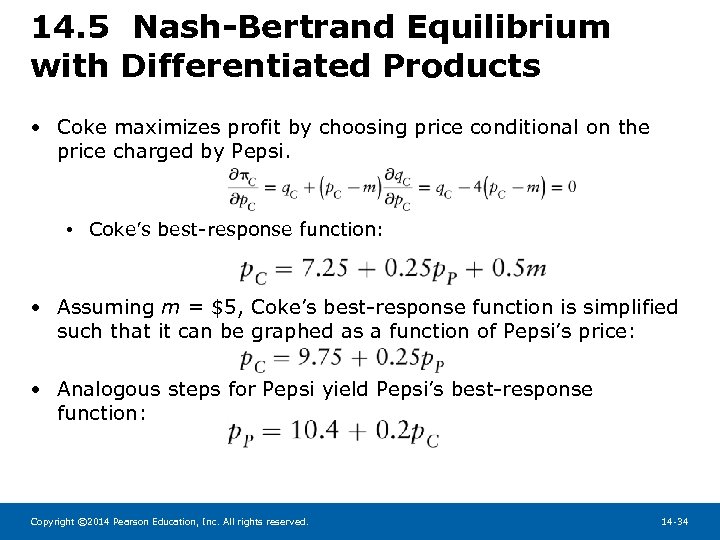 14. 5 Nash-Bertrand Equilibrium with Differentiated Products • Coke maximizes profit by choosing price conditional on the price charged by Pepsi. • Coke’s best-response function: • Assuming m = $5, Coke’s best-response function is simplified such that it can be graphed as a function of Pepsi’s price: • Analogous steps for Pepsi yield Pepsi’s best-response function: Copyright © 2014 Pearson Education, Inc. All rights reserved. 14 -34
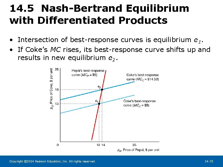 14. 5 Nash-Bertrand Equilibrium with Differentiated Products • Intersection of best-response curves is equilibrium e 1. • If Coke’s MC rises, its best-response curve shifts up and results in new equilibrium e 2. Copyright © 2014 Pearson Education, Inc. All rights reserved. 14 -35
 14. 6 Monopolistic Competition • Monopolistic competition is a market structure in which firms have market power but no additional firm can enter and earn a positive profit. • There are no barriers to entry, so firms enter until economic profits are driven to zero. • What is the difference between competition and monopolistic competition? • The latter face a downward-sloping residual demand curve and can charge a price > MC. • This occurs because they have relatively few rivals or sell differentiated products. Copyright © 2014 Pearson Education, Inc. All rights reserved. 14 -36
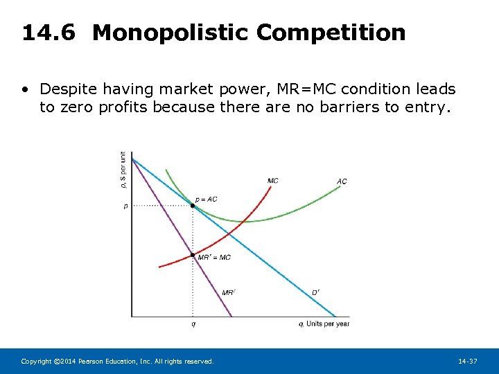 14. 6 Monopolistic Competition • Despite having market power, MR=MC condition leads to zero profits because there are no barriers to entry. Copyright © 2014 Pearson Education, Inc. All rights reserved. 14 -37
 14. 6 Monopolistic Competition • When these firms benefit from economies of scale, each firm is relatively large compared to market demand there is only room for a few firms. • The fewer monopolistically competitive firms, the less elastic is the residual demand curve each firm faces. • The smallest quantity at which AC reaches its minimum is called full capacity or minimum efficient scale. • Monopolistically competitive firm operates at less than full capacity in the long run. Copyright © 2014 Pearson Education, Inc. All rights reserved. 14 -38
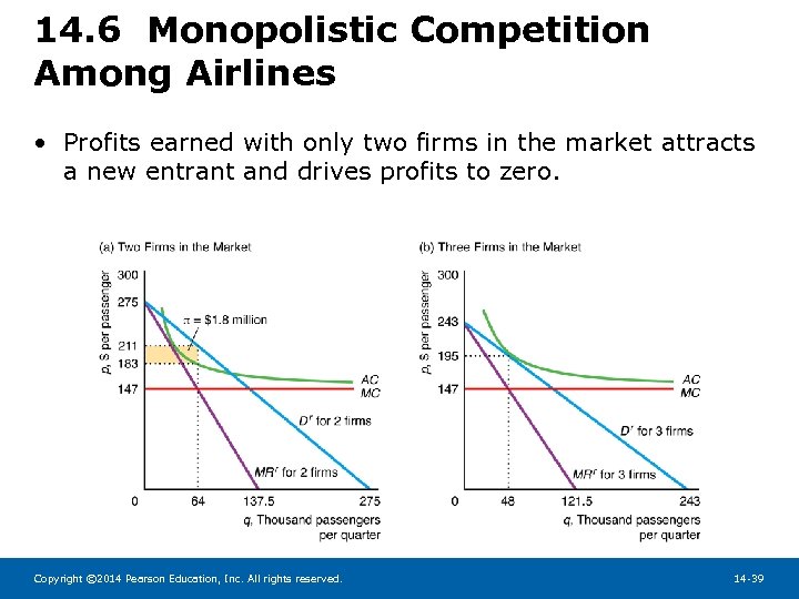 14. 6 Monopolistic Competition Among Airlines • Profits earned with only two firms in the market attracts a new entrant and drives profits to zero. Copyright © 2014 Pearson Education, Inc. All rights reserved. 14 -39
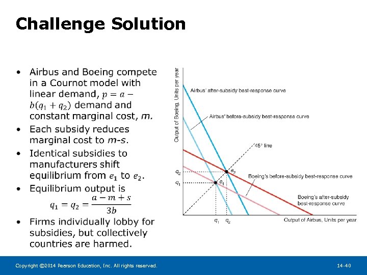 Challenge Solution • Copyright © 2014 Pearson Education, Inc. All rights reserved. 14 -40


