Chapter 14 Multiple Regression Analysis What is

Chapter 14 Multiple Regression Analysis

What is the general purpose of regression? • To model the relationship between the Multiple regression can be used to fit dependent variable y (response) and one or more models to data (predictors or independent variables x with two or more independent variables. explanatory variables) For example, some variation in the price of a house in a large city can be attributed to the size of a house, but there are other variables that also attribute to the price of a house; such as age, lot size, number of bedrooms and bathrooms, etc.

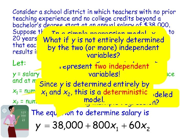Consider a school district in which teachers with no prior teaching experience and no college credits beyond a bachelor’s degree start at an annual salary of $38, 000. Suppose that In a simple regression experience up to for each year of teaching model, x 20 years, the teacher receives an additional $8001 and Whatxif represent two observations y is not entirely determined and postgraduate credit up to 75 credits 2 that each unit of by the two (or more) independent of a single variable. results in an additional $60 per year. In multiplevariables? x 1 and x 2 regression, Let: represent two independent y = salary of a teacher with at most 20 years experience variables! and at most 75 postgraduate units Since y is determined entirely by x 1 = number of years, of experience x 1 and. Howthis is a deterministic x 2 can this scenario be modeled model. x 2 = number of postgraduate units using multiple regression? The equation to determine salary is

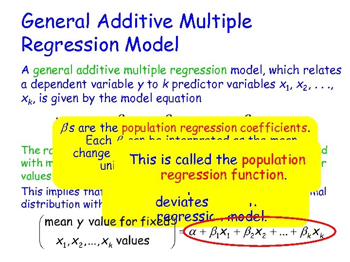General Additive Multiple Regression Model A general additive multiple regression model, which relates a dependent variable y to k predictor variables x 1, x 2, . . . , xk, is given by the model equation b’s are the population regression coefficients. Each bi can be interpreted as the mean The random deviationyewhen the predictor x increase 1 change in is assumed to be normally distributed i with mean value unit and the value of all s forother 0 and. This is called the population standard deviation the any particular regression function. values x 1, …, xk. Remember, remains fixed. predictors this is the amount that a …, xk values, y has This implies that for fixed x 1, x 2, point randomly a normal distribution with standard deviates from the deviation s and regression model.

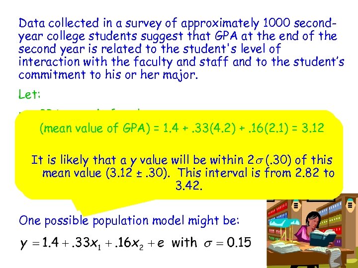Data collected in a survey of approximately 1000 secondyear college students suggest that GPA at the end of the second year is related to the student's level of interaction with the faculty and staff and to the student’s commitment to his or her major. Let: y = GPA at end of sophomore year For sophomores whose level of interaction with the (mean value of GPA) = 1. 4 +. 33(4. 2) +. 16(2. 1) = 3. 12 x 1 = faculty and staff is rated interactionwhose level on a level of faculty and staff at 4. 2 and (measured of scale of 1 to 5) commitment to major is rated at 2. 1, It is likely that a y value will be within 2 s (. 30) of this x 2 = mean of commitment to majorinterval is from 2. 82 to level value (3. 12 ±. 30). This (measured on a scale of (mean +. 33(4. 2) +. 16(2. 1) = 3. 12 1 to 5) value of GPA) = 1. 4 3. 42. One possible population model might be:

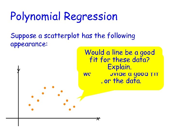Polynomial Regression Suppose a scatterplot has the following appearance: Would a line be a good It looks like a parabola fit for these data? (quadratic function) Explain. would provide a good fit for the data.

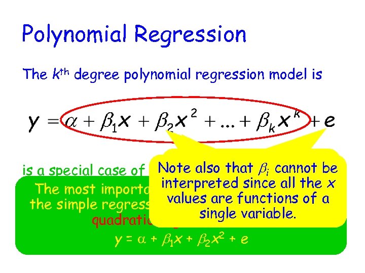Polynomial Regression The kth degree polynomial regression model is Note that we include the Note also that bi cannot be is a special case of therandom deviation e since general multiple interpreted since all regression model with specialis a probabilistic x This is the population regression the The most important this case (other than values when k = functions the function (mean y=value. for fixed 2, x 3, the simple regression 3 modelaremodel. = 1)kisof a x 1 = x, x 2 = x x. xk x single. , variable. values of the predictors). quadratic regression model y = a + b 1 x + b 2 x 2 + e

Many researchers have examined factors that are believed to contribute to the risk of heart attacks. One study found that hip-to-waist ratio was a better predictor of heart attacks than body-mass index. A plot of data from this study of a measure heart-attack risk (y) versus hip-to-waist ratio (x) had a exhibited a curved relationship. A model consistent with summary values given in the paper is Suppose the hip-to-waist ratio is 1. 3, what are the possible values of the heart-attack risk measure (if s = 0. 25)? y = 1. 023 +. 024(1. 3) +. 060(1. 3)2 = 1. 16 It is likely that the heart-attack risk measure for a person with a hip-to-waist ratio of 1. 3 is between. 66 and 1. 66.

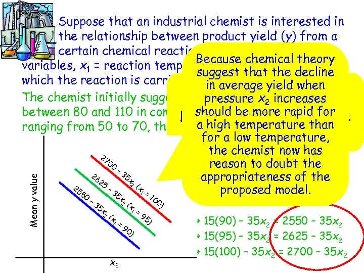Mean y value Suppose that an industrial chemist is interested in the relationship between product yield (y) from a certain chemical reaction and two independent Because chemical theory variables, x 1 = reaction temperature and x 2 = pressure at suggest that the decline which the reaction is carried out. average yield when in Notice each is a straight The chemist initially suggest that with a x 2 increases pressure slope of line for temperatures -35. should be more rapid for between 80 and 110 in combinationlook at plot of these Let’s with pressure values a high temperature than ranging from 50 to 70, the relationship can be modeled by for athree lines. low temperature, the chemist now has 27 00 reason to doubt the – 3 26 5 x appropriateness of the 25 2 ( – 3 55 1 = proposed model. Consider 2 the mean y xvalue for three different particular 5 x 0 10 – 2 ( x temperature 3 values: = 0) 5 x 1 = 90: x 1 = 95: x 1 = 100: 2 (x 95 ) mean 9 value = 1200 + 15(90) – 35 x 2 = 2550 – 35 x 2 =y 0) mean y value = 1200 + 15(95) – 35 x 2 = 2625 – 35 x 2 mean y value = 1200 + 15(100) – 35 x 2 = 2700 – 35 x 2 1 x 2

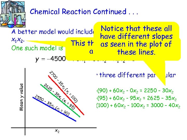Chemical Reaction Continued. . . A better model would include a. Notice that these all third predictor variable have different slopes x 1 x 2. This third predictor variable is as seen in the plot of One such model is an interaction lines. these term. 5 x 2 – 3 Mean y value 00 27 Consider the mean y value for three different particular temperature values: 26 2 5 x 1 = 90: mean y –value = -4500 + 75(90) + 60 x 2 - 0 x 2 = 2250 – 30 x 2 35 x 25 2 ( 50 x 1 = 95: mean y value = -4500 + 75(95) + 60 x 2 - 95 x 2 = 2625 – 35 x 2 x – 3 1 = 5 x x 1 = 100: mean y value = 95) -4500 + 75(100) + 60 x 2 - 100 x 2 = 3000 – 40 x 2 2 (x (x 1 = 0) 10 1 x 2 =9 0)

Interaction Between Variables More than one interaction predictor can be included in the model when more than If the change in the mean y associated with a 1 -unit two independent variable full quadratic, In quadratic regression, the (slope) depends on increase in one independent variables are available. or complete second-order model is: the value of a second independent variable, there is interaction between these two variable. When the variables are denoted by x 1 and x 2, such interaction can be modeled by including x 1 x 2, the product of the variables that interact, as a predictor variable. The general equation for a multiple regression model based on two independent variables x 1 and x 2 that also includes an interaction predictor is

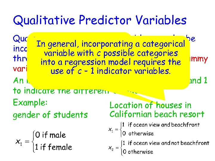Qualitative Predictor Variables Qualitative or categorical variables can also be If ageneral, incorporating a categorical In qualitative variable incorporated three or more regression model had into a multiple variable with c possible categories, indicator variable or through theause of an then into regression model requires the dummy variable. multiple indicator use of c – 1 indicator variables are needed. An indicator variable will use the values of 0 and 1 to indicate the different categories. Example: Location of houses in Californian beach resort gender of students

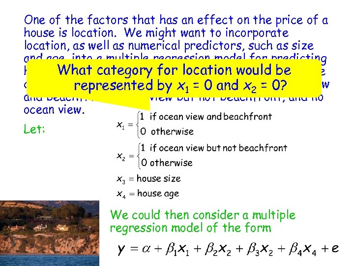One of the factors that has an effect on the price of a house is location. We might want to incorporate location, as well as numerical predictors, such as size and age, into a multiple regression model for predicting house What California beach community houses can be price. category for location would be classified by location into three categories = ocean view represented by x 1 = 0 and x 2 – 0? and beachfront, ocean view but not beachfront, and no ocean view. Let: We could then consider a multiple regression model of the form

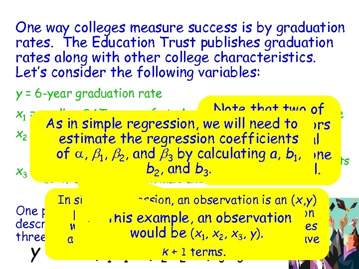One way colleges measure success is by graduation rates. The Education Trust publishes graduation rates along with other college characteristics. Let’s consider the following variables: y = 6 -year graduation rate Note that two of x 1 = median SAT score of students accepted to the college As in simple regression, we these predictors will need to x 2 = student-related expense per full time student (in estimate the regression coefficients are numerical dollars) of a, b 1, b 2, and b 3 by calculating a, and one variables b 1, 1 if college has only female students or only male students b 2, and b 3. is categorical. x 3 = 0 if college has both male and female students In simple regression, an observation is an (x, y) One possible modelmultiple regression, an observation pair. In that would be considered to this example, an and these describe the In consist ofbetween yobservation relationship the k independent variables would three predictors is would be (x 1, x 2– x 3, it would have and the dependent variable , so y). k + 1 terms.

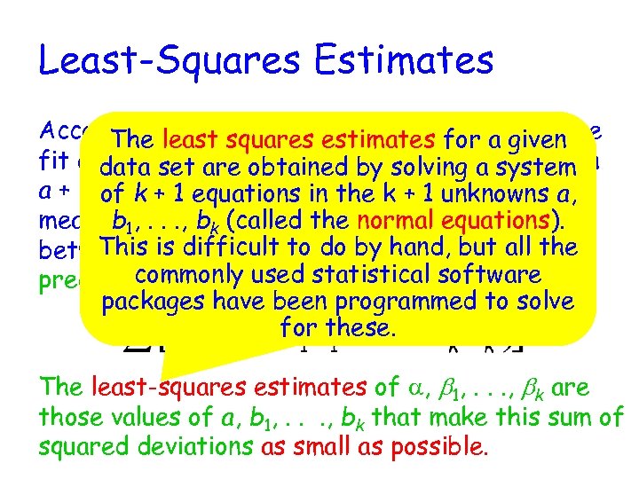Least-Squares Estimates According least squares estimates for a giventhe The to the principles of least-squares, fit ofdata set are obtained by solving a system a particular estimated regression function a + b 1 x 1 +. +. 1 + bkxk to thethe k + 1 unknowns a, of k. equations in observed data is measured. by the sum of the squared deviations b 1, . . , bk (called the normal equations). This is observed y values and but values between thedifficult to do by hand, the yall the commonly used statistical software predicted by the estimated regression function: packages have been programmed to solve y for these. The least-squares estimates of a, b 1, . . . , bk are those values of a, b 1, . . . , bk that make this sum of squared deviations as small as possible.

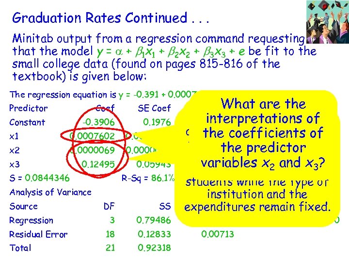Graduation Rates Continued. . . Minitab output from a regression command requesting that the model y = a + b 1 x 1 + b 2 x 2 + b 3 x 3 + e be fit to the small college data (found on pages 815 -816 of the textbook) is given below: The regression equation is y = -0. 391 + 0. 000760 x 1 + 0. 000007 x 2 + 0. 125 x 3 Predictor Coef SE Coef Constant -0. 3906 0. 1976 x 1 0. 0007602 0. 0002300 x 2 0. 0000069 0. 0000045 x 3 0. 12495 0. 05943 S = 0. 0844346 R-Sq = 86. 1% Analysis of Variance Source DF SS 3 0. 79486 Residual Error 18 0. 12833 Total 21 0. 92318 Regression What are. P the T These are the of This value is 0. 064 interpreted interpretations -1. 98 estimates change in as the average for the 6 the coefficients of 3. 30 0. 004 regression for a -year 1. 55 graduation rate the predictor 0. 139 coefficients. x ? 1 unit increase in median variables 0. 050 x 2 enrolling and 3 2. 10 SAT score for students R-Sq(adj) = 83. 8% of while the type institution and the MS F expenditures remain fixed. 0. 26495 0. 00713 37. 16 P 0. 000

Graduation Rates Continued. . . Minitab output from a regression command requesting This = athe x + b x of e be fit to the is + b coefficient + that the model y 1 1 2 2 3 multiple determination. 3 It of the small college data (found on pages 815 -816 textbook) is given, below: This is thethe is s proportion of the e variation in 0. 000760 x 1 + 0. 000007 x 2 + is the The regression equation is y = -0. 391 + estimated standard 6 year This value 0. 125 x 3 graduation rates that canadjusted R 2. Predictor Coef SE T P deviation of the Coef be Constant -1. 98 0. 064 random -0. 3906 explained by the deviation 0. 1976 e. multiple regression model. x 1 0. 0007602 0. 0002300 3. 30 0. 004 x 2 0. 0000069 0. 0000045 1. 55 0. 139 x 3 0. 12495 0. 05943 2. 10 0. 050 S = 0. 0844346 R-Sq = 86. 1% R-Sq(adj) = 83. 8% Analysis of Variance Source DF SS MS F P 3 0. 79486 0. 26495 37. 16 0. 000 Residual Error 18 0. 12833 0. 00713 Total 21 0. 92318 Regression

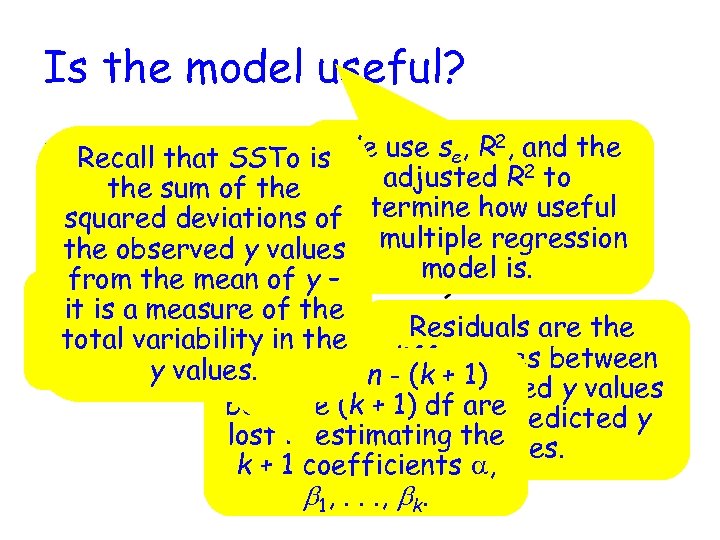Is the model useful? • Recall that SSTo is We use se, deviation The estimate for the random R 2, and the variance s 2 of the by adjusted R 2 to the sum is given determine how useful squared deviations of the observed y values multiple regression model is. from the mean of y – Recall that SSResid is it is a measure of the sum of the squared Residuals are the total variability in the residuals. differences between y values. of multiple determination is The - (k + 1) • The coefficient df = nthe observed y values because (k + 1) df are and the predicted y lost in estimating the values. k + 1 coefficients a, b 1, . . . , bk.

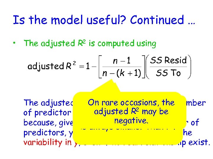Is the model useful? Continued … • The adjusted R 2 is computed using 2 On rare occasions, the The adjusted RBecauseinto account the number takes the value in square brackets important adjusted 22 exceeds of predictor variables. This. Ris may be 1, the value of r adjusted because, given that you negative. number of use a large is always smaller than r 2. predictors, you can account for most of the variability in y, even if no real relationship exist.

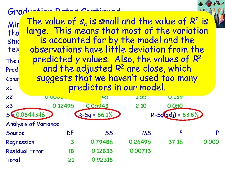Graduation Rates Continued. . . The value of se regression command requesting 2 is Minitab output from a is small and the value of R large. This a + b 1 x + b 2 x + b 3 x + the variation that the model y = means 1 that 2 most 3 ofe be fit to the Is this model useful? is accounted for by the model and small college data (found on pages 815 -816 of thethe textbook) is given Let’s look at these below: observations have little deviation from the 2 predictedthree values again. values + 0. 125 The regression equation is y = -0. 391 + 0. 000760 x 1 + 0. 000007 x 2 of R x 3 y values. Also, the and the adjusted R 2 are T close, which Predictor Coef SE Coef P Constant suggests that we haven’t used too many -0. 3906 0. 1976 -1. 98 0. 064 x 1 0. 0007602 0. 0002300 in our model. 0. 004 3. 30 predictors x 2 x 3 0. 0000069 0. 0000045 0. 12495 S = 0. 0844346 0. 05943 1. 55 0. 139 2. 10 0. 050 R-Sq = 86. 1% R-Sq(adj) = 83. 8% Analysis of Variance Source DF SS MS F P 3 0. 79486 0. 26495 37. 16 0. 000 Residual Error 18 0. 12833 0. 00713 Total 21 0. 92318 Regression

F Distributions • The model utility test for multiple regression is based on a probability distribution called the F distribution. • Like the t and c 2 distributions, the F distributions are based on df. However, it is based upon the df 1 for the numerator of the test statistic and on the df 2 for the denominator of the test statistic. • Each different combination of df 1 and df 2 produces a different F distribution.

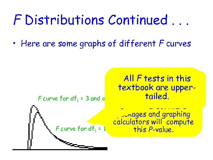F Distributions Continued. . . • Here are some graphs of different F curves The P-value is the this All F tests in area under the associated F textbook are of the curve to the rightupper. F curve for df 1 = 3 and df 2 = 18 calculatedtailed. Most F value. statistical software packages and graphing calculators will compute F curve for df 1 = 18 and df 2 = 3 P-value. this

F Test for Modal Utility Null Hypothesis: H 0: b 1 = b 2 = … = bk = 0 Alternative Hypothesis: At least. SSResid 1, …, bk SSRegr is SSTo - one of b There = no useful linear are not 0 relationship between y and ANY of the predictors. Test Statistic: There is a useful linear relationship between y and at least one of the predictors. Assumptions: For any combination of predictor variables values, the distribution of e is normal with mean 0 and constant variance s 2.

Graduation Rates Continued. . . The model y = a + b 1 x 1 + b 2 x 2 + b 3 x 3 + e was fitted to the small college data (found on pages 815 -816 of the textbook). H 0 : b 1 = b 2 = b 3 = 0 Ha: at least one of the three b’s is not 0 Assumptions: A normal probability plot of the standardized residuals is quite straight, indicating that the assumption of normality of the random deviation distribution is reasonable.

Graduation Rates Continued. . . H 0 : b 1 = b 2 = b 3 = 0 Ha: at least one of the three b’s is not 0 Test Statistic: df 1 = 3, df 2 = 18, a =. 05, P-value ≈ 0 Since P-value < a, we reject H 0. There is evidence to confirm the usefulness of the multiple regression model.

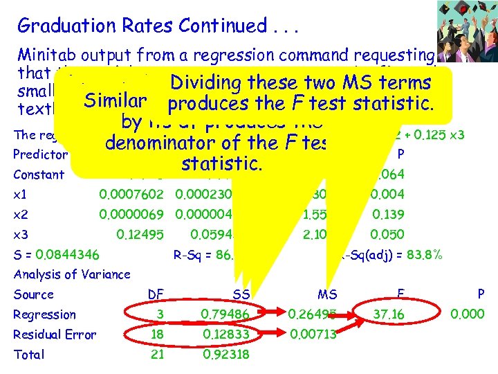Graduation Rates Continued. . . Minitab output from a regression command requesting that the model y = a + b 1 x 1 + b 2 x 2 + b 3 x 3 + e be fit to the Notice the Dividingsquarestwo MS terms sum on these are small college data the SSRegr by its df of the (found of pages 815 -816 Dividing dividing the SSResid Similarly, produces the F given below: textbook) is given the numeratoroftest statistic. producesin the Analysis of the by its df produces the Variance Table. The regression equation is y = -0. 391 + 0. 000760 x 1 + 0. 000007 x 2 + 0. 125 x 3 F test statistic. denominator of the F test Predictor Coef SE Coef T P statistic. Constant -0. 3906 0. 1976 -1. 98 0. 064 x 1 0. 0007602 0. 0002300 3. 30 0. 004 x 2 0. 0000069 0. 0000045 1. 55 0. 139 2. 10 0. 050 x 3 0. 12495 S = 0. 0844346 0. 05943 R-Sq = 86. 1% R-Sq(adj) = 83. 8% Analysis of Variance Source DF SS MS F P 3 0. 79486 0. 26495 37. 16 0. 000 Residual Error 18 0. 12833 0. 00713 Total 21 0. 92318 Regression

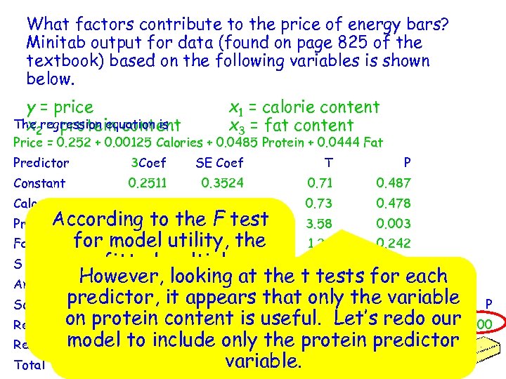What factors contribute to the price of energy bars? Minitab output for data (found on page 825 of the textbook) based on the following variables is shown below. y = price The 2 = protein content x regression equation is x 1 = calorie content x 3 = fat content Price = 0. 252 + 0. 00125 Calories + 0. 0485 Protein + 0. 0444 Fat Predictor 3 Coef SE Coef T P Constant 0. 2511 0. 3524 0. 71 0. 487 0. 001254 0. 001724 0. 73 0. 478 Calories According to Protein 0. 04849 the F test 0. 01353 3. 58 0. 003 for model utility, the Fat 0. 04445 0. 03648 1. 22 0. 242 fitted multiple S = 0. 2789 R-Sq = 74. 7% R-Sq(adj) = 69. 6% Analysis of. However, looking at the t tests for each Variance regression model is predictor, it appears that only the variable P Source useful in predicting the DF SS MS F on redo Regression protein 3 energy bars. 3. 4453 1. 1484 price of thecontent is useful. Let’s 14. 76 our 0. 000 model to include 1. 1670 the 0. 0778 only protein predictor Residual Error 15 variable. Total 18 4. 6122

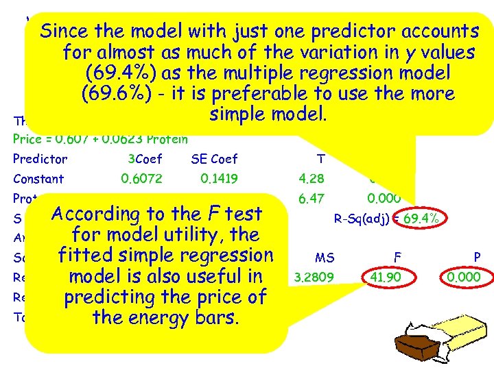What factors contribute to the price of energy bars? Since output for data (found on page 825 of the model with just one predictor accounts Minitab for almost as much of the variation in y values textbook) based on the following variable is shown below. (69. 4%) as the multiple regression model y = price x 2 = protein content (69. 6%) - it is preferable to use the more simple model. The regression equation is Price = 0. 607 + 0. 0623 Protein Predictor 3 Coef SE Coef T P Constant 0. 6072 0. 1419 4. 28 0. 001 0. 062256 0. 009618 6. 47 0. 000 Protein According S = 0. 279843 to the =F test R-Sq 71. 7% for model utility, the Analysis of Variance Source fitted simple regression DF SS Regression 1 3. 2809 model is also useful in Residual predicting the price of Error 17 1. 3313 Total 18 4. 6122 the energy bars. R-Sq(adj) = 69. 4% MS F P 3. 2809 41. 90 0. 000 0. 0763