21edea6364ad5059cb9b94bc1d5dfd7a.ppt
- Количество слайдов: 34
 Chapter 14 Managerial Decision Making Under Uncertainty
 Table of Contents • • • 14 2 14. 1 14. 2 14. 3 14. 4 14. 5 Assessing Risk Attitudes Toward Risk Reducing Risk Investing Under Uncertainty Behavioral Economics and Uncertainty © 2014 Pearson Education, Inc. All rights reserved.
 Introduction • Managerial Problem – The 2010 BP oil spill may cost the firm above $40 billion. However, there is a 1990 law that capped cleanup costs up to $75 million for a rig spill. – How does a cap on liability affect a firm’s willingness to make a risky investment or to invest less than the optimal amount in safety? How does a cap affect the amount of risk that the firm and others in society bear? How does a cap affect th e amount of insurance against the costs of an oil spill that a firm buys? • Solution Approach – We need to focus on how uncertainty affects consumption decisions made by individuals and business decisions made by firms. • Empirical Methods – – 14 3 Probability, expected value and variance are tools for assessing risk. Depending on their attitudes about risk, people and firms try to reduce risk. Investing under uncertainty requires assessing and reducing risk. How psychological factors influence risk assessment is evaluated by behavioral economics. © 2014 Pearson Education, Inc. All rights reserved.
 14. 1 Assessing Risk • A Risk Problem – Gregg, a promoter, is considering whether to schedule an outdoor concert on July 4 th. Booking the concert is a gamble: He stands to make a tidy profit if the weather is good, but he’ll lose a substantial amount if it rains. • Quantifying Risk – This particular event has two possible outcomes: either it rains or it does not rain. – To schedule the concert, first, Gregg quantifies how risky each outcome is using a probability. Second, he uses these probabilities to determine expected earnings. 14 4 © 2014 Pearson Education, Inc. All rights reserved.
 14. 1 Assessing Risk • Probability – Probability: number between 0 and 1 that indicates the likelihood that a particular outcome will occur. – If an outcome cannot occur, probability = 0. If the outcome is sure to happen, probability = 1. If it rains one time in four on July 4 th, probability = ¼ or 25%. – Weather outcomes are mutually exclusive (either it rains or it doesn’t) and exhaustive (no other outcome is possible). So probabilities must add up to 100%. • Calculating Probability using Frequency – Gregg has data about raining on July 4 th : number of years that it rained (n) and the total number of years (N). – Frequency: Ө = n/N 14 5 © 2014 Pearson Education, Inc. All rights reserved.
 14. 1 Assessing Risk • Using Subjective Probability – If Gregg wants to refine the observed frequency, he can use a weather forecaster’s experience to form a subjective probability: best estimate of the likelihood that the outcome will occur—that is, our best, informed guess. – Subjective probability may also be used in the absence of frequency data. • Probability Distributions – A probability distribution relates the probability of occurrence to each possible outcome. – Panel a of Figure 14. 1 shows a probability distribution over five possible outcomes: zero to four days of rain per month in a relatively dry city. – These weather outcomes are mutually exclusive and exhaustive, so exactly one of these outcomes will occur, and the probabilities must add up to 100%. 14 6 © 2014 Pearson Education, Inc. All rights reserved.
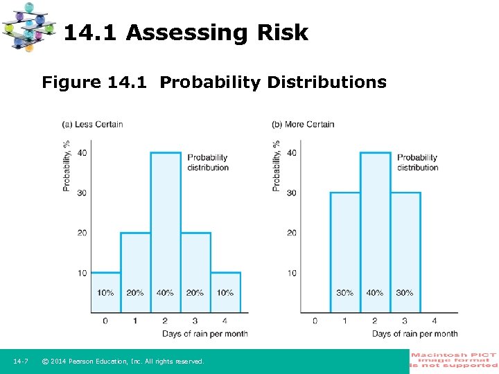 14. 1 Assessing Risk Figure 14. 1 Probability Distributions 14 7 © 2014 Pearson Education, Inc. All rights reserved.
 14. 1 Assessing Risk • Expected Value, EV = Pr 1 V 1 + Pr 2 V 2 + … + Prn. Vn – The expected value, EV, is the weighted average of the values of the outcomes, sum of the product of the probability and the value of each outcome. – Concert and rain example: EV = [0. 5 *15]+[0. 5*( 5)] = 5 – Gregg will earn an average of 5 per concert over a long period of time. • Variance, 2= Pr 1(V 1 – EV)2 + Pr 2(V 2 – EV)2 + … + Prn(Vn – EV)2 – Variance, 2: measures the spread of the probability distribution; probability weighted average of the squares of the differences between the observed outcome and the expected value. – Concert and rain example: Variance = [0. 5 (15 5)2] + [0. 5 ( 5 5)2] = 100 – Another measure of risk is the standard deviation, : square root of the variance. – For the outdoor concert, the values are 2 = 100 and = 10. 14 8 © 2014 Pearson Education, Inc. All rights reserved.
 14. 2 Attitudes Towards Risk • Expected Utility: EU = Pr 1 x U (V 1) + Pr 2 x U (V 2) + … + Prn x U (Vn) – Expected utility: probability weighted average of the utility from each possible outcome. – For example, Gregg’s EU = [0. 5 U(15)] + [0. 5 U( 5)] – EU and EV have similar math form. The key difference is that the EU captures the tradeoff between risk and value, whereas the EV considers only value. • Fair Bet and Risk Attitudes – We can classify people based on their willingness to make a fair bet: a bet with an expected value of zero. – Someone who is unwilling to make a fair bet is risk averse. – A person who is indifferent about making a fair bet is risk neutral. – A person who will make a fair bet is risk preferring. 14 9 © 2014 Pearson Education, Inc. All rights reserved.
 14. 2 Attitudes Towards Risk • Risk Aversion – A concave utility function shows diminishing marginal utility of wealth: The extra pleasure from each extra dollar of wealth is smaller than the extra pleasure from the previous dollar. – A concave utility function shows risk aversion: unwillingness to take a fair bet. • Unwillingness to Take a Fair Bet – Irma’s utility function is concave, her subjective probability is 50% (Figure 14. 2). – Irma can keep $40 (secure action) or buy a stock (riskier action). Buying the stock is a fair bet because its EV = (0. 5 x $70 + 0. 5 x $10) = $40 (same as keeping $40). – However, Irma does not accept the fair bet (risk averse). The secure utility at point b is higher than EU of buying the stock at point d (120 > 105). – A risk averse person picks the less risky choice if both choices have the same EV. • Using Calculus: Diminishing Marginal Utility of Wealth – Irma’s utility from Wealth is U(W); Marginal Utility = d. U(W)/d. W > 0 – Diminishing marginal utility cocondition (concavity): d 2 U(W)/d. W 2 < 0 14 10 © 2014 Pearson Education, Inc. All rights reserved.
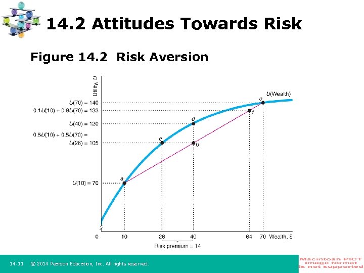 14. 2 Attitudes Towards Risk Figure 14. 2 Risk Aversion 14 11 © 2014 Pearson Education, Inc. All rights reserved.
 14. 2 Attitudes Towards Risk • Risk Premium – The risk premium is the maximum amount that a decision maker would pay to avoid taking a risk. – Equivalently, the risk premium is the minimum extra compensation (premium) that a decision maker would require to willingly incur a risk. • Risk Premium Calculation – Risk premium: the difference between the expected value of the uncertain prospect and the certainty equivalent – Certainty Equivalent: if held with certainty, would yield the same utility as the uncertain prospect (point e in Figure 14. 2). – The risk premium in Figure 14. 2 is 14 (40 – 26). – Irma would accept to buy the stock (fair bet) if offered $14 to do it. 14 12 © 2014 Pearson Education, Inc. All rights reserved.
 14. 2 Attitudes Towards Risk • Risk Neutrality – A risk neutral person is indifferent about taking a fair bet. – Such a person has a constant marginal utility of wealth: Each extra dollar of wealth raises utility by the same amount as the previous dollar. – The utility function is a straight line in a graph of utility against wealth. – As a consequence, a risk neutral person’s utility depends only on wealth and not on risk. • Risk Neutrality Calculation – In panel a of Figure 14. 3, Irma’s utility is a straight line, constant marginal utility of wealth (35/30). – Her expected utility of a fair bet (between points a and c) exactly equals her utility with certain wealth of 40 (at point b). – A risk neutral person chooses the option with the highest expected value, because maximizing expected value maximizes utility. The risk premium is zero. 14 13 © 2014 Pearson Education, Inc. All rights reserved.
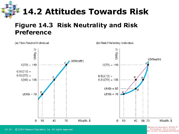 14. 2 Attitudes Towards Risk Figure 14. 3 Risk Neutrality and Risk Preference 14 14 © 2014 Pearson Education, Inc. All rights reserved.
 14. 2 Attitudes Towards Risk • Risk Preference – An individual with an increasing marginal utility of wealth is risk preferring: willing to take a fair bet. – Increasing marginal utility of wealth: the extra pleasure from each extra dollar of wealth is bigger than the extra pleasure from the previous dollar. – The utility function is convex. • Risk Preference Calculation and Risk Premium – If Irma has the utility function in panel b of Figure 14. 3, she is risk preferring. Her expected utility from buying the stock, 105 at b, is higher than her certain utility if she does not buy the stock, 82 at d. Therefore, she buys the stock. – A risk preferring person is willing to pay for the right to make a fair bet (a negative risk premium). Irma would like to pay no more than $18 (40 – 58). 14 15 © 2014 Pearson Education, Inc. All rights reserved.
 14. 2 Attitudes Towards Risk • Risk Attitudes of Managers – Some shareholders want managers to be risk neutral and to maximize expected profit. However, managers may make risk averse or risk preferring decisions. • Managers Act in Their Own Interests (Principal Agent Problem) – If a manager is worried about being fired if the firm has large losses, the manager may act to avoid the possibility of such losses. The firm is made to pay a risk premium (reduced expected profit) to avoid an extreme risk of losing money. – If the manager’s compensation is based on the firm’s short run profit and there is no penalty in the event of a very bad outcome, the manager may prefer risk. • Shareholders May Want Managers to be Risk Averse – If bankruptcy would impose large costs on shareholders, they might prefer that managers try to avoid bankruptcy even at the expense of reduced expected profit. 14 16 © 2014 Pearson Education, Inc. All rights reserved.
 14. 3 Reducing Risk • All Individuals and Firms Want to Reduce Risk – Risk averse, risk neutral, and risk preferring people all reduce risk of unfair bets. – Individuals can avoid optional risky activities, but often they can’t escape risk altogether. • Abstaining as an Easy Way of Reducing Risk – The simplest way to avoid risk is to abstain from optional risky activities (lottery, stock market, high risk jobs). – Even when you can’t avoid risk altogether, you can take precautions to reduce the probability of bad events or the magnitude of any loss that might occur (closing doors at home, installing fire alarms, servicing a car regularly). • Strategies to Reduce Risk – Three most common ways: obtaining information, diversification, and insurance 14 17 © 2014 Pearson Education, Inc. All rights reserved.
 14. 3 Reducing Risk • Obtaining Information – Collecting accurate information before acting is one of the most important ways in which people can reduce risk and increase expected value and expected utility. • An Application to Bond Ratings – Investors look at Moody’s and Standard & Poor’s ratings. Their letter grade ratings reflect whether a bond’s issuer has made timely payments in the past, whether the issuer is in danger of becoming bankrupt, and other problems. – Investment grade bonds (Moody Baa through Aaa or Standard and Poor BBB through AAA) are said to be suitable for purchase by an institutional money manager (legally obligated to be a prudent investor). – Lower ranked bonds (Moody C through Ba and Standard and Poor D through BB+) are riskier and must offer higher rates of return to attract buyers. – The lowest ranked, junk bonds are generally issued by new firms. 14 18 © 2014 Pearson Education, Inc. All rights reserved.
 14. 3 Reducing Risk • “Don’t Put All Your Eggs in One Basket” – This common advice is called technically risk pooling or diversification • Correlation and Diversification – How much diversification reduces risk depends on the degree to which the payoffs of various investments are correlated (move in the same direction). – If the performances of two investments move independently—do not move together in a predictable way—their payoffs are uncorrelated. • Perfect Negative Correlation to Eliminate Risk – Diversification can eliminate risk if the returns to two investments are perfectly negatively correlated. – Case: Two firms compete for a government contract with equal chance of winning. You can buy 2 shares of stock in either firm for $20. The stock of the firm that wins the contract will be worth $40, whereas the stock of the loser will be worth $10 (perfect negative correlation). Why diversify? – Buying two shares of the same stock: EV = 0. 5 x 80 + 0. 5 x 20 = 50 and 2 = 900 – Buying one share of each firm: EV = 0. 5 x 50 + 0. 5 x 50 = 50 but 2 = 0. Zero risk. 14 19 © 2014 Pearson Education, Inc. All rights reserved.
 14. 3 Reducing Risk • No Correlation and Risk Reduction – Diversification reduces risk even if the two investments are uncorrelated or imperfectly positively correlated, but cannot be eliminated. – Case: Same case as before but whether one firm wins (W) a contract does not affect whether the other firm loses (L). There are 4 scenarios (WW, WL, LW, LL), each with probability ¼ or 25%. – Buying one share of each firm: EV = 0. 25 x 80 + 0. 5 x 50 + 0. 25 x 20 = 50, 2 = 450. Same EV but the risk has been reduced by half. • Positive Correlation and Risk Reduction – Diversification can reduce risk even if the investments are positively correlated provided that the correlation is not perfect. – Diversification does not reduce risk if two investments have a perfect positive correlation. – Case: Same case as before but both firms win or lose together (perfectly positively correlated). The EV and the 2 are the same whether you buy two shares of one firm or one share of each firm. 14 20 © 2014 Pearson Education, Inc. All rights reserved.
 14. 3 Reducing Risk • Diversification Through Mutual Funds – One way to effectively own shares in a number of companies at once and diversify is by buying shares in a mutual fund. For instance the S&P 500, which is a value weighted average of 500 large firms’ stocks. – Mutual funds allow investors to reduce the risk associated with uncorrelated price movements across stocks. Random, firm specific risks are reduced. • Diversification Cannot Eliminate Systemic Market Risk – A stock mutual fund has a market wide risk, a risk that is common to the overall market. Prices of almost all stocks tend to rise when the economy is expanding and to fall when the economy is contracting. – No investor can avoid the systematic risks associated with shifts in the economy that have a similar effect on most stocks even if you buy a diversified stock mutual fund. Even the global economy has a global market wide risk. 14 21 © 2014 Pearson Education, Inc. All rights reserved.
 14. 3 Reducing Risk • Insurance – Many individuals and firms buy insurance to shift some or all of the risk they face to an insurance company. Global insurance revenues exceeded $4. 59 trillion in 2011, approximately 6% of world GDP. – A risk averse person or firm pays an insurance premium to the insurance company in exchange for an amount of money if a bad outcome occurs. • Determining the Amount of Insurance to Buy – Case: Scott is risk averse, wants to insure his store that is worth 500. Probability of fire is 20%. If a fire occurs, the store will be worth nothing. – With no insurance, the EV = 0. 8 x 500 + 0. 2 x 0 = 400, and 2 = 10, 000 – Fair Insurance: a contract between an insurer and a policyholder in which the expected value of the contract to the policyholder is zero (fair bet). – With fair insurance, for every 1 dollar of insurance premium paid, the company will pay Scott 5 dollars to cover the damage if the fire occurs, so that he has 1 dollar less if the fire does not occur, but 4 dollars more if it does occur. – Scott’s premium x to make his wealth 400 in either case: 500 – x = 4 x, x = 100. – With insurance, the EV = 400 and 2 = 0. Zero risk. 14 22 © 2014 Pearson Education, Inc. All rights reserved.
 14. 3 Reducing Risk • Fairness and Insurance – Because insurance firms have operating expenses, we expect that real world insurance companies offer unfair insurance: the expected payout to policyholders is less than the premiums paid by policyholders. – A risk averse person fully insures if offered a fair insurance. If not, buy less. – A monopoly insurance company could charge an amount up to the risk premium a person is willing to pay to avoid risk. If there were more firms, it would be lower but still enough to cover operating expenses. • Insurance and Diversifiable Risks – By pooling the risks of many people, the insurance company can lower its risk much below that of any individual. – Insurance companies generally try to protect themselves from insolvency (going bankrupt) by selling policies only for risks that they can adequately diversify. – Because wars are nondiversifiable risks, insurance companies normally do not offer policies insuring against wars. 14 23 © 2014 Pearson Education, Inc. All rights reserved.
 14. 4 Investing Under Uncertainty • Risk Neutral Investing – Chris is a risk neutral monopoly owner. Because she is risk neutral, she invests if the EV of the firm rises due to the investment. Any action that increases her EV must also increase her EU because she is indifferent to risk. – In panel a of Figure 14. 4, if Chris does not open the new store, she makes $0. If she does open the new store, she expects to make $200 (thousand) with 80% probability and to lose $100 (thousand) with 20% probability. • Solution – Chris decides whether to invest or not at the decision node (rectangle). The circle, a chance node, denotes that a random process determines the outcome. – Chris decides to invest because EV = 140 > 0. She prefers an EV of 140 to a certain one of 0. 14 24 © 2014 Pearson Education, Inc. All rights reserved.
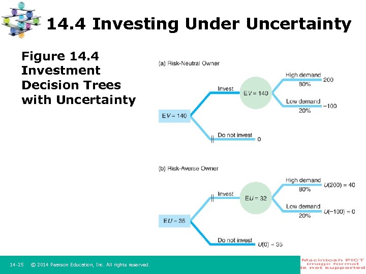 14. 4 Investing Under Uncertainty Figure 14. 4 Investment Decision Trees with Uncertainty 14 25 © 2014 Pearson Education, Inc. All rights reserved.
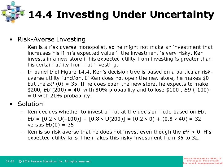 14. 4 Investing Under Uncertainty • Risk Averse Investing – Ken is a risk averse monopolist, so he might not make an investment that increases his firm’s expected value if the investment is very risky. Ken invests in a new store if his expected utility from investing is greater than his certain utility from not investing. – In panel b of Figure 14. 4, Ken’s decision tree is based on a particular risk averse utility function. If Ken does not open the new store, he makes $0 but the EU (0) = 35. If he does open the new store, he expects to make $200, EU (200) = 40 with 80% probability and to lose $100 , EU ( 100) = 0 with 20% probability. • Solution – Ken decides whether to invest or not at the decision node based on EU. – EU = [0. 2 U(– 100)] + [0. 8 U(200)] = (0. 2 0) + (0. 8 40) = 32 versus EU(0) = 35 – Ken is so risk averse that he does not invest even though the EV > 0. His expected utility falls if he makes this risky investment from 35 to 32. 14 26 © 2014 Pearson Education, Inc. All rights reserved.
 14. 5 Behavioral Economics and Uncertainty • Biased Assessment and Probabilities – People often have mistaken beliefs about the probability that an event will occur. – Why? We consider false beliefs about causality and overconfidence. • The Gambler’s Fallacy – Gambler’s fallacy: false belief that past events affect current, independent outcomes. – Case: You flip a fair coin and it comes up heads six times in a row. What are the odds that you’ll get a tail on the next flip? Because past flips do not affect this one, the chance of a tail remains 50%. Yet, some people believe that a head is much more likely because they are on a “run, ” or less likely because a tail is “due. ” • Overconfidence – Another common explanation for why some people make bets that the rest of us avoid is overconfidence. – Evidence: Many U. S. high school basketball and football players believe they will get an athletic scholarship to attend college, but less than 5% receive one. Of this elite group, about 25% expect to become professional athletes, but only about 1. 5% succeed. 14 27 © 2014 Pearson Education, Inc. All rights reserved.
 14. 5 Behavioral Economics and Uncertainty • Violations of Expected Utility Theory – Some people’s choices violate the basic assumptions of expected utility theory. – Why? People change choices depending on how questions are framed or have biases about certainty. • Framing and Reflection Effect – Framing matters – Reflection effect: attitudes toward risk are reversed (reflected) for gains versus losses. People are often risk averse when making choices involving gains, but they are often risk preferring when making choices involving losses. • The Certainty Effect – Many people put excessive weight on outcomes that they consider to be certain relative to risky outcomes. 14 28 © 2014 Pearson Education, Inc. All rights reserved.
 14. 6 Behavioral Economics and Uncertainty • Prospect Theory – According to prospect theory, people are concerned about gains and losses (changes in wealth) rather than the level of wealth, as in expected utility theory. – People start with a reference point (base level of wealth) and think about alternative outcomes as gains or losses relative to that reference level. • Comparing Expected Utility and Prospect Theories – Case: Muzhe and Rui have initial wealth W. They may choose a gamble where they get a loss of A with probability or a gain of B with probability 1 – . – Muzhe’s decision with expected utility: EU = U(W+A) + (1 – )U(W+B). If EU > U(W). – Rui’s decision with prospect theory: the reference level is the current wealth W with a value V(0). The values of the gamble V(A) and V(B) have decision weights w( ) and w(1 ). So, if V(0) < [w( ) V(A) + w(1 ) V(B)] Rui gambles. 14 29 © 2014 Pearson Education, Inc. All rights reserved.
 14. 6 Behavioral Economics and Uncertainty • Value Function in Prospect Theory – Prospect theory proposes a value function, V, that has an S shape (Figure 14. 6) • Properties of the Value Function – 1 st, the curve passes through the reference point at the origin: gains and losses are determined relative to the initial situation where there is no gain or loss. – 2 nd, both sections of the curve are concave to the horizontal, outcome axis: more sensitive to changes of small losses or gains than large ones. – 3 rd, the curve is asymmetric with respect to gains and losses: The S curve in Figure 14. 6 shows that people suffer more from a loss than they benefit from a comparable size gain. – The value function reflects loss aversion: people dislike making losses more than they like making gains. 14 30 © 2014 Pearson Education, Inc. All rights reserved.
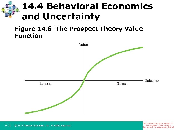 14. 4 Behavioral Economics and Uncertainty Figure 14. 6 The Prospect Theory Value Function 14 31 © 2014 Pearson Education, Inc. All rights reserved.
 Managerial Solution • Managerial Problem – How does a cap on liability affect a firm’s willingness to make a risky investment or to invest less than the optimal amount in safety? How does a cap affect the amount of risk that the firm and others in society bear? How does a cap affect th e amount of insurance against the costs of an oil spill that a firm buys? • Solution – Oil spills have a subjective probability to occur. Firms invest in oil rigs if the EV > 0 and this depends on the value of . If is low, most likely oil firms will invest. The cap on liability causes risk neutral and risk averse firms to invest, accepting higher probability for oil spills. – A limit on liability increases the economy’s total risk if it encourages the drilling company to drill when it would not otherwise. – If the drilling company’s liability is capped, it buys insurance only for the non capped amount and it does not fully insure. Society will be responsible for the extra damages if the spill occurs. 14 32 © 2014 Pearson Education, Inc. All rights reserved.
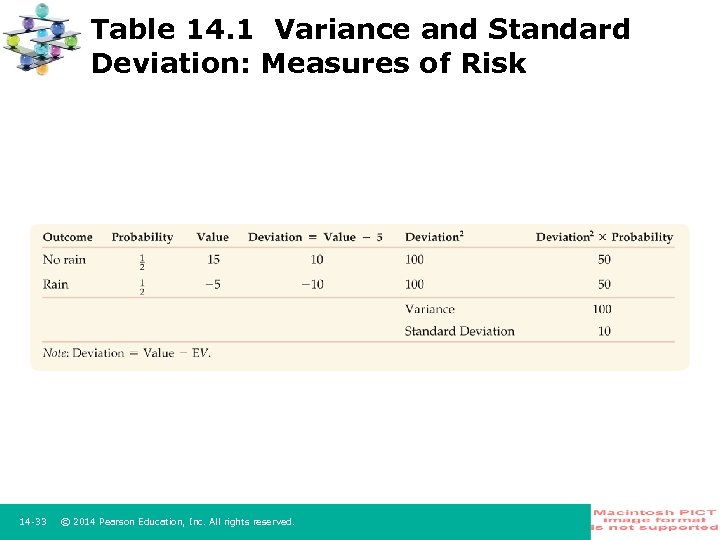 Table 14. 1 Variance and Standard Deviation: Measures of Risk 14 33 © 2014 Pearson Education, Inc. All rights reserved.
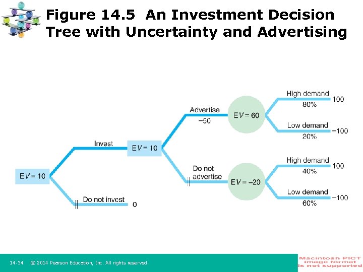 Figure 14. 5 An Investment Decision Tree with Uncertainty and Advertising 14 34 © 2014 Pearson Education, Inc. All rights reserved.


