Chapter 14 Advanced Pricing Techniques Mc Graw-Hill Irwin Copyright

Chapter 14: Advanced Pricing Techniques Mc. Graw-Hill/Irwin Copyright © 2011 by the Mc. Graw-Hill Companies, Inc. All rights reserved.

Advanced Pricing Techniques • Price discrimination • Multiple products • Cost-plus pricing 14 -2

Capturing Consumer Surplus • Uniform pricing • Charging the same price for every unit of the product • Price discrimination • More profitable alternative to uniform pricing • Market conditions must allow this practice to be profitably executed • Technique of charging different prices for the same product • Used to capture consumer surplus (turning consumer surplus into profit) 14 -3

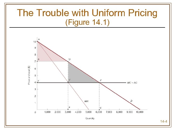The Trouble with Uniform Pricing (Figure 14. 1) 14 -4

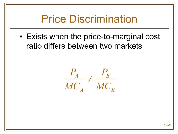Price Discrimination • Exists when the price-to-marginal cost ratio differs between two markets 14 -5

Price Discrimination Three conditions necessary to practice price discrimination profitably: 1) Firm must possess some degree of market power 2) A cost-effective means of preventing resale between lower- and higher-price buyers (consumer arbitrage) must be implemented 3) Price elasticities must differ between individual buyers or groups of buyers 14 -6

First-Degree (Perfect) Price Discrimination • Every unit is sold for the maximum price each consumer is willing to pay • Allows the firm to capture entire consumer surplus • Difficulties • Requires precise knowledge about every buyer’s demand for the good • Seller must negotiate a different price for every unit sold to every buyer 14 -7

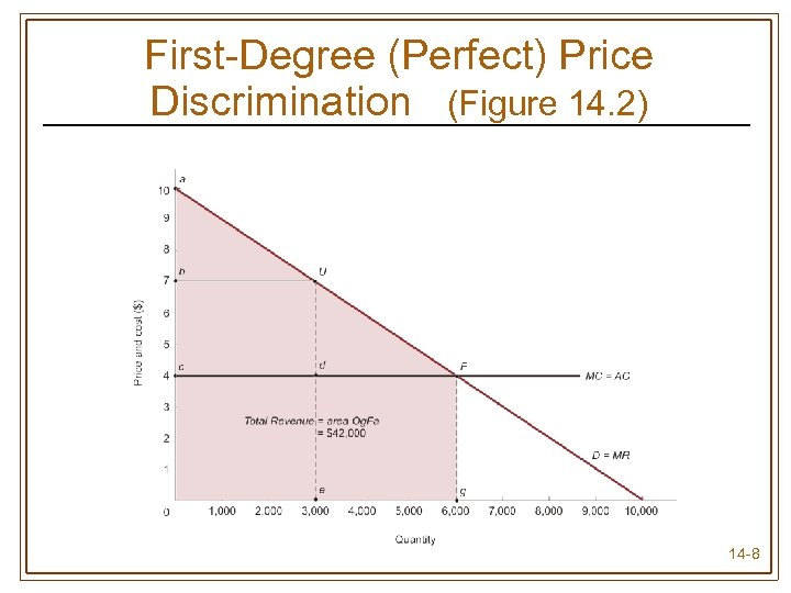First-Degree (Perfect) Price Discrimination (Figure 14. 2) 14 -8

Second-Degree Price Discrimination • Lower prices are offered for larger quantities and buyers can self-select the price by choosing how much to buy • When the same consumer buys more than one unit of a good or service at a time, the marginal value placed on additional units declines as more units are consumed 14 -9

Examples of Second Degree Price Discrimination • Two-part pricing • Block pricing 14 -10

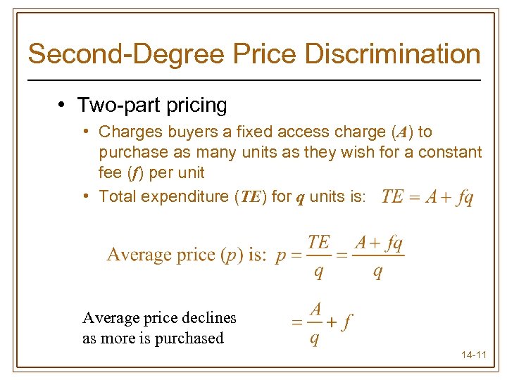Second-Degree Price Discrimination • Two-part pricing • Charges buyers a fixed access charge (A) to purchase as many units as they wish for a constant fee (f) per unit • Total expenditure (TE) for q units is: Average price declines as more is purchased 14 -11

Second-Degree Price Discrimination • When consumers have identical demands, entire consumer surplus can be captured by: • Setting f *= MC • Setting A* = consumer surplus (CS) • Optimal usage fee when two groups of buyers have identical demands is the level for which MRf = MCf 14 -12

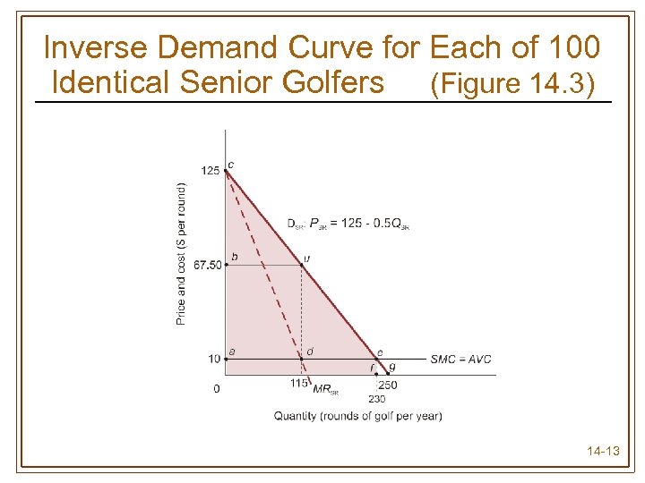Inverse Demand Curve for Each of 100 Identical Senior Golfers (Figure 14. 3) 14 -13

Summary of Two Part Pricing • Consumers will purchase product until marginal benefit = unit price • Unit price will at least cover marginal cost • With consumers with different preferences unit price will be above marginal cost • Consumers will choose to purchase as long as consumer surplus given unit price is greater than lump-sum fee (right to purchase) • With identical preferences monopolist will capture the entire consumer surplus • With different preferences some consumers will retain part of their consumer surplus 14 -14

Second-Degree Price Discrimination • Declining block pricing • Offers quantity discounts over successive discrete blocks of quantities purchased 14 -16

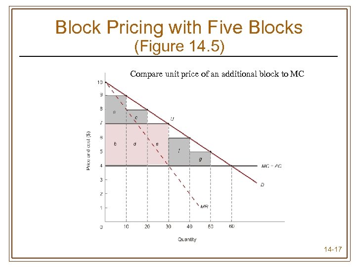Block Pricing with Five Blocks (Figure 14. 5) Compare unit price of an additional block to MC 14 -17

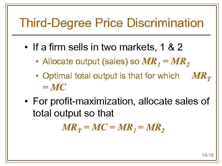Third-Degree Price Discrimination • If a firm sells in two markets, 1 & 2 • Allocate output (sales) so MR 1 = MR 2 • Optimal total output is that for which MRT = MC • For profit-maximization, allocate sales of total output so that MRT = MC = MR 1 = MR 2 14 -18

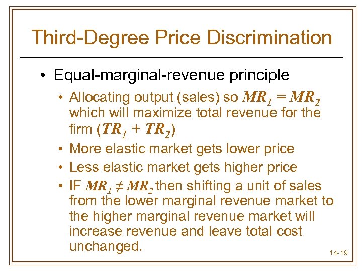Third-Degree Price Discrimination • Equal-marginal-revenue principle • Allocating output (sales) so MR 1 = MR 2 which will maximize total revenue for the firm (TR 1 + TR 2) • More elastic market gets lower price • Less elastic market gets higher price • IF MR 1 ≠ MR 2 then shifting a unit of sales from the lower marginal revenue market to the higher marginal revenue market will increase revenue and leave total cost unchanged. 14 -19

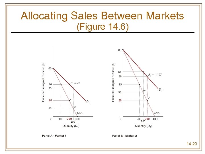Allocating Sales Between Markets (Figure 14. 6) 14 -20

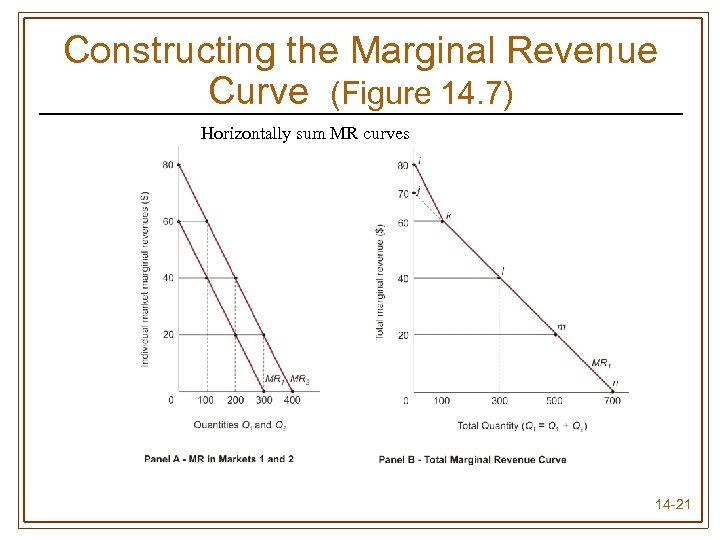Constructing the Marginal Revenue Curve (Figure 14. 7) Horizontally sum MR curves 14 -21

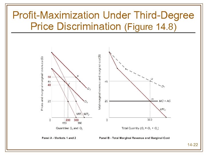Profit-Maximization Under Third-Degree Price Discrimination (Figure 14. 8) 14 -22

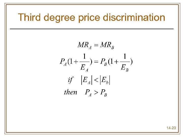Third degree price discrimination 14 -23

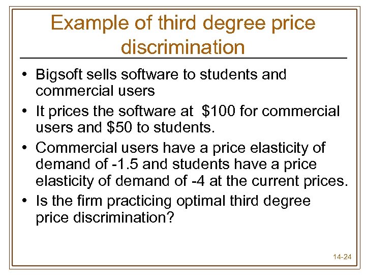Example of third degree price discrimination • Bigsoft sells software to students and commercial users • It prices the software at $100 for commercial users and $50 to students. • Commercial users have a price elasticity of demand of -1. 5 and students have a price elasticity of demand of -4 at the current prices. • Is the firm practicing optimal third degree price discrimination? 14 -24

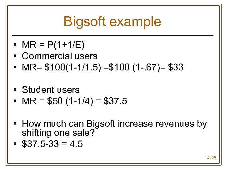Bigsoft example • MR = P(1+1/E) • Commercial users • MR= $100(1 -1/1. 5) =$100 (1 -. 67)= $33 • Student users • MR = $50 (1 -1/4) = $37. 5 • How much can Bigsoft increase revenues by shifting one sale? • $37. 5 -33 = 4. 5 14 -25

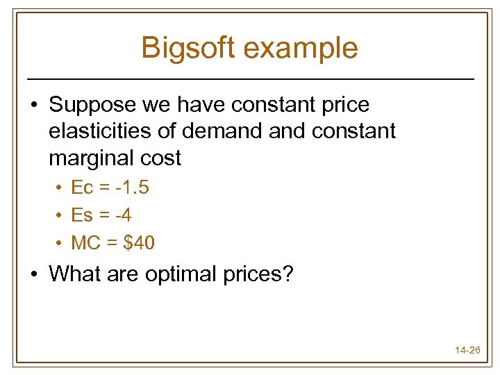Bigsoft example • Suppose we have constant price elasticities of demand constant marginal cost • Ec = -1. 5 • Es = -4 • MC = $40 • What are optimal prices? 14 -26

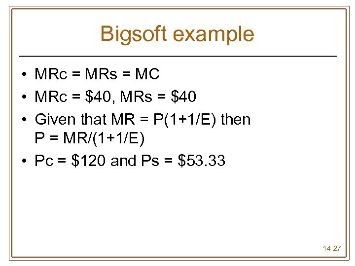Bigsoft example • MRc = MRs = MC • MRc = $40, MRs = $40 • Given that MR = P(1+1/E) then P = MR/(1+1/E) • Pc = $120 and Ps = $53. 33 14 -27

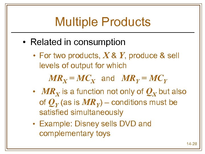Multiple Products • Related in consumption • For two products, X & Y, produce & sell levels of output for which MRX = MCX and MRY = MCY • MRX is a function not only of QX but also of QY (as is MRY) – conditions must be satisfied simultaneously • Example: Disney sells DVD and complementary toys 14 -28

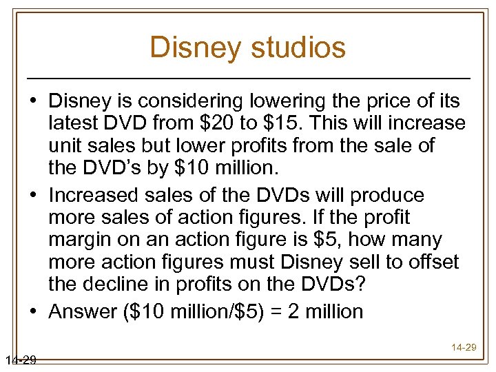Disney studios • Disney is considering lowering the price of its latest DVD from $20 to $15. This will increase unit sales but lower profits from the sale of the DVD’s by $10 million. • Increased sales of the DVDs will produce more sales of action figures. If the profit margin on an action figure is $5, how many more action figures must Disney sell to offset the decline in profits on the DVDs? • Answer ($10 million/$5) = 2 million 14 -29

Multiple Products • Related in production as substitutes • For two products, X & Y, allocate production facility so that MRPX = MRPY • Optimal level of facility usage in the long run is where MRPT = MC • For profit-maximization: MRPT = MC = MRPX = MRPY 14 -30

JBL Plastics • JBL has a vacuum press that can produce plastic cars or tanks. • The marginal cost of producing two cars or one tank is $5. • The marginal revenue from the sale of a toy car is $3 and the price is $6. • The marginal revenue from the sale of a toy tank is $7 and the price is $14. • MRPc from toy cars is $3 x 2= $6 • MRPt from toy tanks is $7 x 1=$7 • Should JBL readjust the ratio of cars to tanks it is producing so that MRPt= MRPc= MC 14 -31

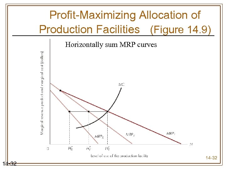Profit-Maximizing Allocation of Production Facilities (Figure 14. 9) Horizontally sum MRP curves 14 -32

Multiple Products • Related in production as complements • To maximize profit, set joint marginal revenue equal to marginal cost: MRJ = MC • If profit-maximizing level of joint production exceeds output where MRJ kinks, units beyond zero MR are disposed of rather than sold • Profit-maximizing prices are found using demand functions for the two goods 14 -33

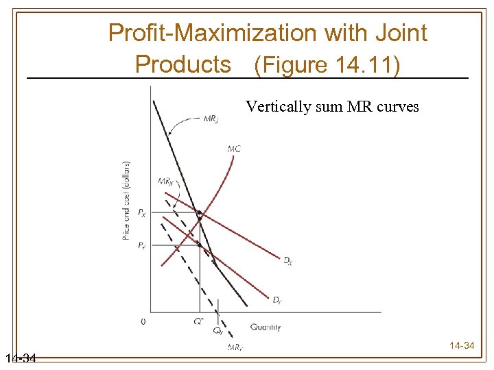Profit-Maximization with Joint Products (Figure 14. 11) Vertically sum MR curves 14 -34

Farmer Jones • The marginal revenue from another cow brought to market includes marginal revenue of $300 from the sale of beef at a price of $500 and a price of $50 and marginal revenue $25 from the sale of the hide. • If the marginal cost of bringing another cow to market is $350, should he slaughter another cow? 14 -35

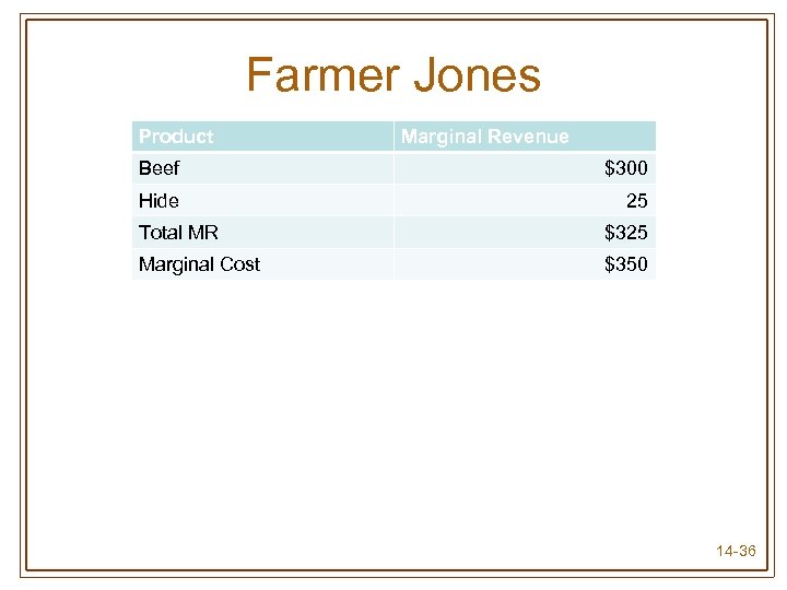Farmer Jones Product Marginal Revenue Beef $300 Hide 25 Total MR $325 Marginal Cost $350 14 -36

Bundling Multiple Products • When price discrimination is not possible, bundling multiple goods and charging a single price can be more profitable than charging individual prices for multiple goods • Two conditions for profitable bundling • Consumers must have different demand prices for each good in the bundle • Demand prices must be negatively correlated across consumer types 14 -37

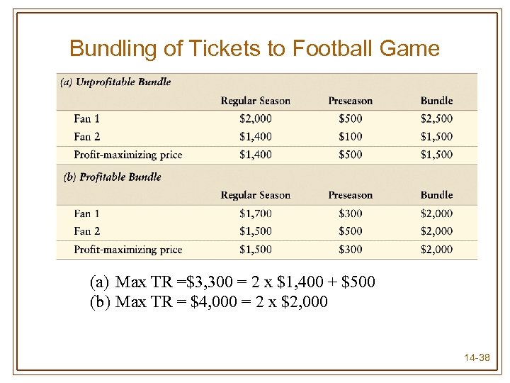Bundling of Tickets to Football Game (a) Max TR =$3, 300 = 2 x $1, 400 + $500 (b) Max TR = $4, 000 = 2 x $2, 000 14 -38

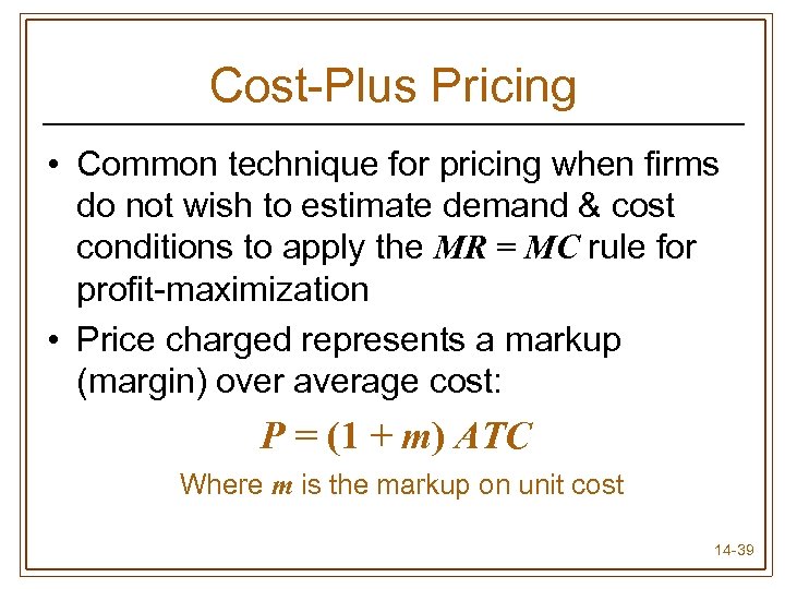Cost-Plus Pricing • Common technique for pricing when firms do not wish to estimate demand & cost conditions to apply the MR = MC rule for profit-maximization • Price charged represents a markup (margin) over average cost: P = (1 + m) ATC Where m is the markup on unit cost 14 -39

Cost-Plus Pricing • Does not generally produce profitmaximizing price • Fails to incorporate information on demand & marginal revenue • Uses average, not marginal, cost 14 -40

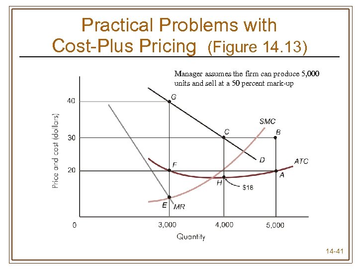Practical Problems with Cost-Plus Pricing (Figure 14. 13) Manager assumes the firm can produce 5, 000 units and sell at a 50 percent mark-up 14 -41

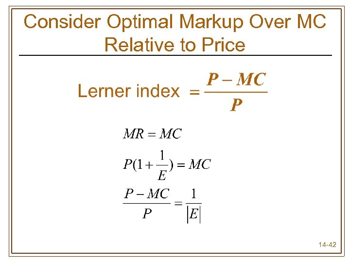Consider Optimal Markup Over MC Relative to Price 14 -42