a1c01335255533d0c7c8b4cbe49bee62.ppt
- Количество слайдов: 112
Chapter 13 Exchange Rates, Business Cycles, and Macroeconomic Policy in the Open Economy
Chapter Outline • Exchange Rates • How Exchange Rates Are Determined: A Supply-and-Demand Analysis • The IS-LM Model for an Open Economy • Macroeconomic Policy in an Open Economy with Flexible Exchange Rates • Fixed Exchange Rates Copyright © 2014 Pearson Education 13 -2
Exchange Rates • Nominal exchange rates – The nominal exchange rate tells you how much foreign currency you can obtain with one unit of the domestic currency • For example, if the nominal exchange rate is 90 yen per dollar, one dollar can be exchanged for 90 yen • Transactions between currencies take place in the foreign exchange market • Denote the nominal exchange rate (or simply, exchange rate) as enom in units of the foreign currency per unit of domestic currency Copyright © 2014 Pearson Education 13 -3

Exchange Rates • Nominal exchange rates – Under a flexible-exchange-rate system or floating-exchange-rate system, exchange rates are determined by supply and demand may change every day; this is the current system for major currencies Copyright © 2014 Pearson Education 13 -4
Exchange Rates • Nominal exchange rates – In the past, many currencies operated under a fixed-exchange-rate system, in which exchange rates were determined by governments • The exchange rates were fixed because the central banks in those countries offered to buy or sell the currencies at the fixed exchange rate • Examples include the gold standard, which operated in the late 1800 s and early 1900 s, and the Bretton Woods system, which was in place from 1944 until the early 1970 s • Even today, though major currencies are in a flexibleexchange-rate system, some smaller countries fix their exchange rates Copyright © 2014 Pearson Education 13 -5
How Exchange Rates Are Determined • In touch with data and research: Exchange rates – Trading in currencies occurs around-the-clock, since some market is open in some country any time of day – The spot rate is the rate at which one currency can be traded for another immediately – The forward rate is the rate at which one currency can be traded for another at a fixed date in the future (for example, 30, 90, or 180 days from now) – A pattern of rising forward rates suggests that people expect the spot rate to be rising in the future Copyright © 2014 Pearson Education 13 -6
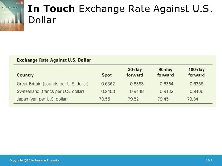
In Touch Exchange Rate Against U. S. Dollar Copyright © 2014 Pearson Education 13 -7

Exchange Rates • Real exchange rates – The real exchange rate tells you how much of a foreign good you can get in exchange for one unit of a domestic good – If the nominal exchange rate is 80 yen per dollar, and it costs 800 yen to buy a hamburger in Tokyo compared to 2 dollars in New York, the price of a U. S. hamburger relative to a Japanese hamburger is 0. 2 Japanese hamburgers per U. S. hamburger Copyright © 2014 Pearson Education 13 -8

Exchange Rates • Real exchange rates – The real exchange rate is the price of domestic goods relative to foreign goods, or e = enom P/PFor (13. 1) – To simplify matters, we’ll assume that each country produces a unique good – In reality, countries produce many goods, so we must use price indexes to get P and PFor – If a country’s real exchange rate is rising, its goods are becoming more expensive relative to the goods of the other country Copyright © 2014 Pearson Education 13 -9

Exchange Rates • Appreciation and depreciation – In a flexible-exchange-rate system, when enom falls, the domestic currency has undergone a nominal depreciation (or it has become weaker); when enom rises, the domestic currency has become stronger and has undergone a nominal appreciation – In a fixed-exchange-rate system, a weakening of the currency is called a devaluation, a strengthening is called a revaluation – We also use the terms real appreciation and real depreciation to refer to changes in the real exchange rate (Summary 15) Copyright © 2014 Pearson Education 13 -10
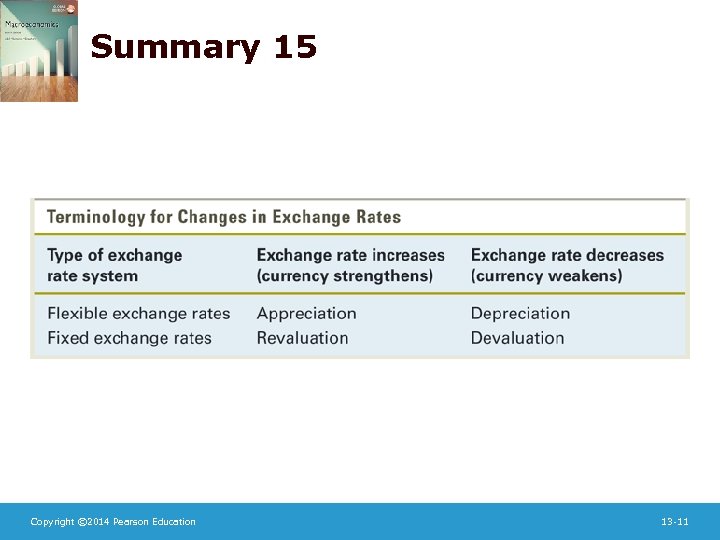
Summary 15 Copyright © 2014 Pearson Education 13 -11

Exchange Rates • Purchasing power parity – To examine the relationship between the nominal exchange rate and the real exchange rate, think first about a simple case in which all countries produce the same goods, which are freely traded • If there were no transportation costs, the real exchange rate would have to be e = 1, or else everyone would buy goods where they were cheaper Copyright © 2014 Pearson Education 13 -12

Exchange Rates • Purchasing power parity – Setting e = 1 in Eq. (13. 1) gives P = PFor/enom – (13. 2) This means that similar goods have the same price in terms of the same currency, a concept known as purchasing power parity, or PPP Copyright © 2014 Pearson Education 13 -13
Exchange Rates • Purchasing power parity – Empirical evidence PPP holds in the long run but not in the short run Countries produce different goods Some goods aren’t traded Transportation costs Legal barriers to trade Copyright © 2014 Pearson Education 13 -14

Exchange Rates • Purchasing Power Parity – When PPP doesn’t hold, using Eq. (13. 1), we can decompose changes in the real exchange rate into parts Δe/e = Δenom/enom + ΔP/P – ΔPFor/PFor – This can be rearranged as Δenom/enom = Δe/e + πFor – π Copyright © 2014 Pearson Education (13. 3) 13 -15

Exchange Rates • Purchasing Power Parity – Thus a nominal appreciation is due to a real appreciation or a lower rate of inflation than in the foreign country Copyright © 2014 Pearson Education 13 -16
Exchange Rates • Purchasing Power Parity – In the special case in which the real exchange rate doesn’t change, so that Δe/e = 0, the resulting equation in Eq. (13. 3) is called relative purchasing power parity, since nominal exchange-rate movements reflect only changes in inflation • Relative purchasing power parity works well as a description of exchange-rate movements in highinflation countries, since in those countries, movements in relative inflation rates are much larger than movements in real exchange rates Copyright © 2014 Pearson Education 13 -17

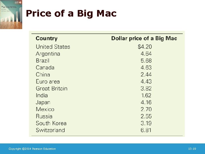
Exchange Rates • In touch with data and research: Mc. Parity – As a test of the PPP hypothesis, the Economist magazine periodically reports on the prices of Big Mac hamburgers in different countries – The prices, when translated into dollar terms using the nominal exchange rate, range from $1. 62 in India to $6. 81 in Switzerland (using 2012 data), so PPP definitely doesn’t hold Copyright © 2014 Pearson Education 13 -18
Price of a Big Mac Copyright © 2014 Pearson Education 13 -19
Exchange Rates • In touch with data and research: Mc. Parity – The hamburger price data forecast movements in exchange rates • Hamburger prices might be expected to converge, so countries in which Big Macs are expensive may have a depreciation, while countries in which Big Macs are cheap may have an appreciation Copyright © 2014 Pearson Education 13 -20
Exchange Rates • The real exchange rate and net exports – The real exchange rate (also called the terms of trade) is important because it represents the rate at which domestic goods and services can be traded for those produced abroad • An increase in the real exchange rate means people in a country can get more foreign goods for a given amount of domestic goods Copyright © 2014 Pearson Education 13 -21
Exchange Rates • The real exchange rate and net exports – The real exchange rate also affects a country’s net exports (exports minus imports) • Changes in net exports have a direct impact on export and import industries in the country • Changes in net exports affect overall economic activity and are a primary channel through which business cycles and macroeconomic policy changes are transmitted internationally Copyright © 2014 Pearson Education 13 -22
Exchange Rates • The real exchange rate and net exports – The real exchange rate affects net exports through its effect on the demand for goods • A high real exchange rate makes foreign goods cheap relative to domestic goods, so there’s a high demand foreign goods (in both countries) • With demand foreign goods high, net exports decline • Thus the higher the real exchange rate, the lower a country’s net exports Copyright © 2014 Pearson Education 13 -23
Exchange Rates • The real exchange rate and net exports – The J curve • The effect of a change in the real exchange rate may be weak in the short run and can even go the “wrong” way • Although a rise in the real exchange rate will reduce net exports in the long run, in the short run it may be difficult to quickly change imports and exports • As a result, a country will import and export the same amount of goods for a time, with lower relative prices on the foreign goods, thus increasing net exports Copyright © 2014 Pearson Education 13 -24

Exchange Rates • The real exchange rate and net exports – The J curve • Similarly, a real depreciation will lead to a decline in net exports in the short run and a rise in the long run • This pattern of net exports is known as the J curve (Fig. 13. 1) Copyright © 2014 Pearson Education 13 -25
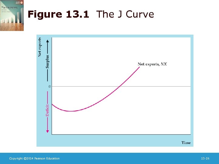
Figure 13. 1 The J Curve Copyright © 2014 Pearson Education 13 -26

Exchange Rates • The real exchange rate and net exports – The J curve • The analysis in this chapter assumes a time period long enough that the movements along the J curve are complete, so that a real depreciation raises net exports and a real appreciation reduces net exports Copyright © 2014 Pearson Education 13 -27
How Exchange Rates Are Determined: A Supply-and-Demand Analysis • What causes changes in the exchange rate? – To analyze this, we’ll use supply-and-demand analysis, assuming a fixed price level – Holding prices fixed means that changes in the real exchange rate are matched by changes in the nominal exchange rate Copyright © 2014 Pearson Education 13 -28

How Exchange Rates Are Determined • What causes changes in the exchange rate? – The nominal exchange rate is determined in the foreign exchange market by supply and demand for the currency – Demand supply are plotted against the nominal exchange rate, just like demand supply for any good (Fig. 13. 3) Copyright © 2014 Pearson Education 13 -29
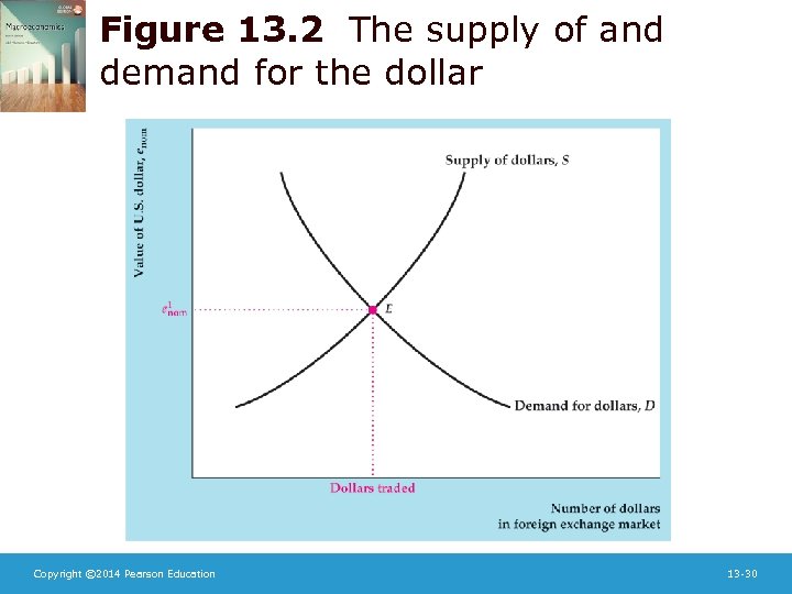
Figure 13. 2 The supply of and demand for the dollar Copyright © 2014 Pearson Education 13 -30

How Exchange Rates Are Determined • What causes changes in the exchange rate? – Supplying dollars means offering dollars in exchange for the foreign currency – The supply curve slopes upward, because if people can get more units of foreign currency for a dollar, they’ll supply more dollars – Demanding dollars means wanting to buy dollars in exchange for the foreign currency – The demand curve slopes downward, because if people need to give up a greater amount of foreign currency to obtain one dollar, they’ll demand fewer dollars Copyright © 2014 Pearson Education 13 -31

How Exchange Rates Are Determined • Why do people demand or supply dollars? – People need dollars for two reasons: • To be able to buy U. S. goods and services (U. S. exports) • To be able to buy U. S. real and financial assets (U. S. financial inflows) – These transactions are the two main categories in the balance of payments accounts: the current account and the capital and financial account Copyright © 2014 Pearson Education 13 -32

How Exchange Rates Are Determined • Why do people demand or supply dollars? – People want to sell dollars for two reasons: • To be able to buy foreign goods and services (U. S. imports) • To be able to buy foreign real and financial assets (U. S. financial outflows) Copyright © 2014 Pearson Education 13 -33
How Exchange Rates Are Determined • Factors that increase demand for U. S. exports and assets will increase demand for dollars, shifting the demand curve to the right and increasing the nominal exchange rate – For example, an increase in the quality of U. S. goods relative to foreign goods will lead to an appreciation of the dollar (Fig. 13. 4) Copyright © 2014 Pearson Education 13 -34

Figure 13. 3 The effect of increased export quality on the value of the dollar Copyright © 2014 Pearson Education 13 -35
How Exchange Rates Are Determined • Macroeconomic determinants of the exchange rate and net export demand – Look at how changes in real output or the real interest rate are linked to the exchange rate and net exports, to develop an open-economy IS-LM model Copyright © 2014 Pearson Education 13 -36
How Exchange Rates Are Determined • Macroeconomic determinants of the exchange rate and net export demand – Effects of changes in output (income) • A rise in domestic output (income) raises demand for goods and services, including imports, so net exports decline • To increase purchases of imports, people must sell the domestic currency to buy foreign currency, increasing the supply of foreign currency, which reduces the exchange rate • The opposite occurs if foreign output (income) rises – Domestic net exports rise – The exchange rate appreciates Copyright © 2014 Pearson Education 13 -37

How Exchange Rates Are Determined • Macroeconomic determinants of the exchange rate and net export demand – Effects of changes in real interest rates • A rise in the domestic real interest rate (with the foreign real interest rate held constant) causes foreigners to want to buy domestic assets, increasing the demand for domestic currency and raising the exchange rate • The rise in the exchange rate leads to a decline in net exports • The opposite occurs if the foreign real interest rate rises – Domestic net exports rise – The exchange rate depreciates Copyright © 2014 Pearson Education 13 -38

Summary 16 Copyright © 2014 Pearson Education 13 -39

Summary 17 Copyright © 2014 Pearson Education 13 -40
The IS-LM Model for an Open Economy • Only the IS curve is affected by having an open economy instead of a closed economy; the LM curve and FE line are the same – Note that we don’t use the AD-AS model because we need to know what happens to the real interest rate, which has an important impact on the exchange rate – The IS curve is affected because net exports are part of the demand for goods – The IS curve remains downward sloping Copyright © 2014 Pearson Education 13 -41
The IS-LM Model for an Open Economy • Any factor that shifts the closed-economy IS curve shifts the open-economy IS curve in the same way • Factors that change net exports (given domestic output and the domestic real interest rate) shift the IS curve – Factors that increase net exports shift the IS curve up and to the right – Factors that decrease net exports shift the IS curve down and to the left Copyright © 2014 Pearson Education 13 -42
The IS-LM Model for an Open Economy • The open-economy IS curve – The goods-market equilibrium condition is Sd – Id = NX (13. 4) • This means that desired foreign lending must equal foreign borrowing Copyright © 2014 Pearson Education 13 -43
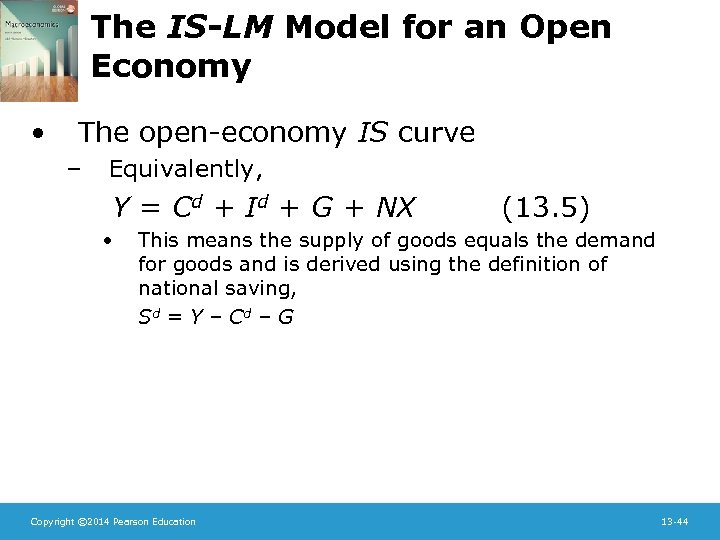
The IS-LM Model for an Open Economy • The open-economy IS curve – Equivalently, Y = Cd + Id + G + NX • (13. 5) This means the supply of goods equals the demand for goods and is derived using the definition of national saving, Sd = Y – Cd – G Copyright © 2014 Pearson Education 13 -44
The IS-LM Model for an Open Economy • The open-economy IS curve – Plotting Sd – Id and NX illustrates goods-market equilibrium (Fig. 13. 5) Copyright © 2014 Pearson Education 13 -45

Figure 13. 4 Goods market equilibrium in an open economy Copyright © 2014 Pearson Education 13 -46
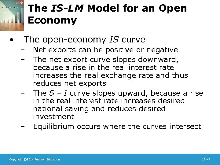
The IS-LM Model for an Open Economy • The open-economy IS curve – – Net exports can be positive or negative The net export curve slopes downward, because a rise in the real interest rate increases the real exchange rate and thus reduces net exports The S – I curve slopes upward, because a rise in the real interest rate increases desired national saving and reduces desired investment Equilibrium occurs where the curves intersect Copyright © 2014 Pearson Education 13 -47

The IS-LM Model for an Open Economy • The open-economy IS curve – To get the open-economy IS curve, we need to see what happens when domestic output changes (Fig. 13. 6) Copyright © 2014 Pearson Education 13 -48
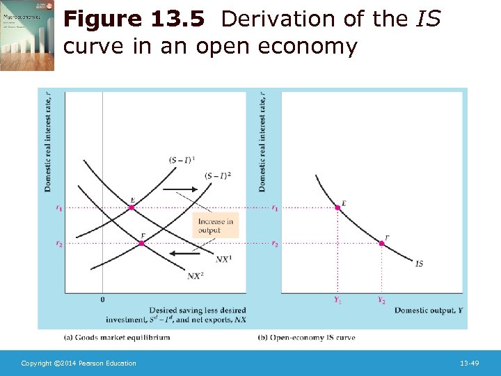
Figure 13. 5 Derivation of the IS curve in an open economy Copyright © 2014 Pearson Education 13 -49
The IS-LM Model for an Open Economy • The open-economy IS curve – – – Higher output increases saving, so the S – I curve shifts to the right Higher output reduces net exports, so the NX curve shifts to the left The new equilibrium occurs at a lower real interest rate, so the IS curve is downward sloping Copyright © 2014 Pearson Education 13 -50
The IS-LM Model for an Open Economy • Factors that shift the open-economy IS curve – Any factor that raises the real interest rate that clears the goods market at a constant level of output shifts the IS curve up and to the right • An example is a temporary increase in government purchases (Fig. 13. 7) Copyright © 2014 Pearson Education 13 -51
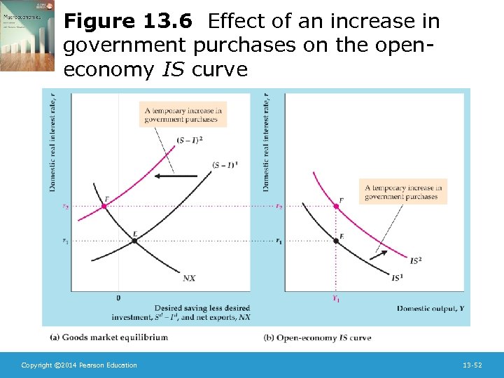
Figure 13. 6 Effect of an increase in government purchases on the openeconomy IS curve Copyright © 2014 Pearson Education 13 -52

The IS-LM Model for an Open Economy • Factors that shift the open-economy IS curve – – The rise in government purchases reduces desired national saving, shifting the S – I curve to the left, shifting the IS curve up and to the right Anything that reduces desired national saving relative to investment shifts the IS curve up and to the right Copyright © 2014 Pearson Education 13 -53
The IS-LM Model for an Open Economy • Factors that shift the open-economy IS curve – Anything that raises a country’s net exports, given domestic output and the domestic real interest rate, will shift the open-economy IS curve up and to the right (Fig. 13. 8) Copyright © 2014 Pearson Education 13 -54
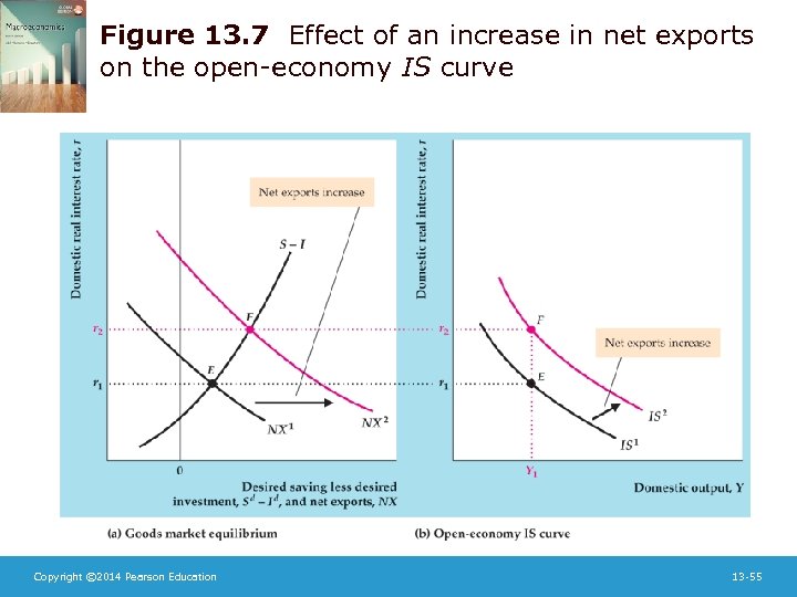
Figure 13. 7 Effect of an increase in net exports on the open-economy IS curve Copyright © 2014 Pearson Education 13 -55
The IS-LM Model for an Open Economy • Factors that shift the open-economy IS curve – – The increase in net exports is shown as a shift to the right in the NX curve This raises the real interest rate for a fixed level of output, shifting the IS curve up and to the right Copyright © 2014 Pearson Education 13 -56

The IS-LM Model for an Open Economy • Factors that shift the open-economy IS curve – Three things could increase net exports for a given level of output and real interest rate • • • An increase in foreign output, which increases foreigners’ demand for domestic exports An increase in the foreign real interest rate, which makes people want to buy foreign assets, causing the exchange rate to depreciate, which in turn causes net exports to rise A shift in worldwide demand toward the domestic country’s goods, for example, as occurs if the quality of domestic goods improves Copyright © 2014 Pearson Education 13 -57

Summary 18 Copyright © 2014 Pearson Education 13 -58

The IS-LM Model for an Open Economy • The international transmission of business cycles – The impact of foreign economic conditions on the real exchange rate and net exports is one of the principal ways by which cycles are transmitted internationally Copyright © 2014 Pearson Education 13 -59
The IS-LM Model for an Open Economy • The international transmission of business cycles – What would be the effect on Japan of a recession in the United States? • • • – The decline in U. S. output would reduce demand for Japanese exports, shifting the Japanese IS curve down and to the left In a Keynesian model, or in the classical misperceptions model, this leads to recession in Japan In a classical (RBC) model, the decline in net exports wouldn’t affect Japanese output A similar effect could occur because of a shift in preferences (or trade restrictions) for Japanese goods Copyright © 2014 Pearson Education 13 -60
Macroeconomic Policy in an Open Economy with Flexible Exchange Rates • Two key questions – How do fiscal and monetary policy affect a country’s real exchange rate and net exports? – How do the macroeconomic policies of one country affect the economies of other countries? Copyright © 2014 Pearson Education 13 -61
Macroeconomic Policy • Three steps in analyzing these questions – Use the domestic economy’s IS-LM diagram to see the effects on domestic output and the domestic real interest rate – See how changes in the domestic real interest rate and output affect the exchange rate and net exports – Use the foreign economy’s IS-LM diagram to see the effects of domestic policy on foreign output and the foreign real interest rate Copyright © 2014 Pearson Education 13 -62

Macroeconomic Policy • A fiscal expansion – Look at a temporary increase in domestic government purchases using the classical (RBC) model • The rise in government purchases shifts the IS curve up and to the right and the FE line to the right (Fig. 13. 9) Copyright © 2014 Pearson Education 13 -63
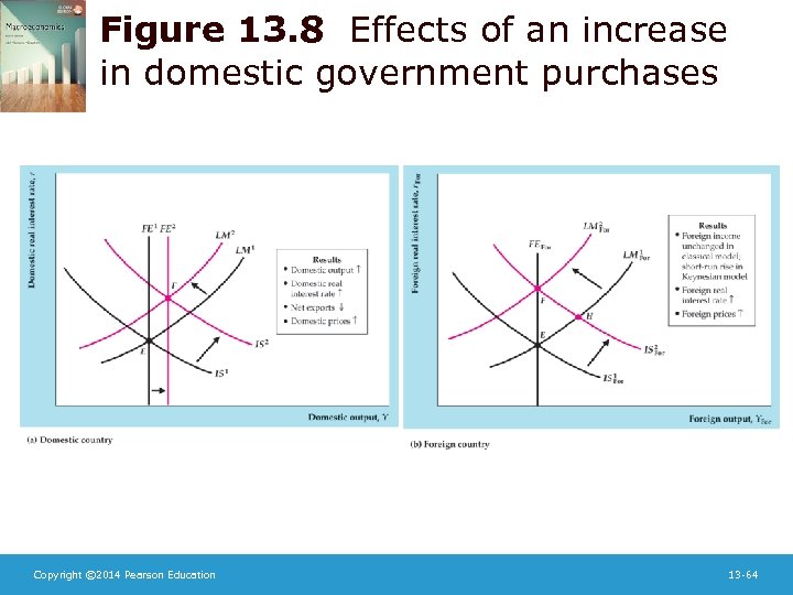
Figure 13. 8 Effects of an increase in domestic government purchases Copyright © 2014 Pearson Education 13 -64
Macroeconomic Policy • A fiscal expansion – The LM curve shifts up and to the left to restore equilibrium as the price level rises – Both the real interest rate and output rise in the domestic country – Higher output reduces the exchange rate, while a higher real interest rate increases the exchange rate, so the effect on the exchange rate is ambiguous – Higher output and a higher real interest rate both reduce net exports, supporting the twin deficits idea Copyright © 2014 Pearson Education 13 -65

Macroeconomic Policy • A fiscal expansion – How do these changes affect a foreign country’s economy? • The decline in net exports for the domestic economy means a rise in net exports for the foreign country, so the foreign country’s IS curve shifts up and to the right • In the classical model, the LM curve shifts up and to the left as the price level rises to restore equilibrium, thus raising the foreign real interest rate, but foreign output is unchanged • In a Keynesian model, the shift of the IS curve would give the foreign country higher output temporarily Copyright © 2014 Pearson Education 13 -66

Macroeconomic Policy • A fiscal expansion – In either the classical or Keynesian model, a temporary increase in domestic government purchases raises domestic income (temporarily) and the domestic real interest rate, as in a closed economy • It also reduces domestic net exports, so government spending crowds out both investment and net exports • The effect on the exchange rate is ambiguous • The foreign real interest rate and price level rise • In the Keynesian model, foreign output rises temporarily Copyright © 2014 Pearson Education 13 -67

Macroeconomic Policy • A monetary contraction – Look at a reduction in the domestic money supply in a Keynesian model – Short-run effects on the domestic and foreign economies (Fig. 13. 10) Copyright © 2014 Pearson Education 13 -68

Figure 13. 09 Effects of a decrease in the domestic money supply Copyright © 2014 Pearson Education 13 -69
Macroeconomic Policy • A monetary contraction – The domestic LM curve shifts up and to the left – In the short run, domestic output is lower and the real interest rate is higher – The exchange rate appreciates, because lower output reduces demand for imports, thus reducing the supply of the domestic currency to the foreign exchange market, and because a higher real interest rate increases demand for the domestic currency Copyright © 2014 Pearson Education 13 -70

Macroeconomic Policy • A monetary contraction – How are net exports affected? • The decline in domestic income reduces domestic demand foreign goods, tending to increase net exports • The rise in the real interest rate leads to an appreciation of the domestic currency and tends to reduce net exports • Following the J curve analysis, assume the latter effect is weak in the short run, so that net exports increase Copyright © 2014 Pearson Education 13 -71

Macroeconomic Policy • A monetary contraction – How is the foreign country affected? • Since domestic net exports increase, foreign net exports must decrease, shifting the foreign IS curve down and to the left • Output and the real interest rate in the foreign country decline • So a domestic monetary contraction leads to recession abroad Copyright © 2014 Pearson Education 13 -72

Macroeconomic Policy • A monetary contraction – Long-run effects on the domestic and foreign economies • In the long run, wages and prices in the domestic economy decline and the LM curve returns to its original position • All real variables, including net exports and the real exchange rate, return to their original levels • As a result, the foreign IS curve returns to its original level as well • Thus there is no long-run effect on any real variables, either domestically or abroad Copyright © 2014 Pearson Education 13 -73

Macroeconomic Policy • A monetary contraction – Long-run effects on the domestic and foreign economies • This result holds in the long run in the Keynesian model, but it holds immediately in the classical (RBC) model; monetary contraction affects only the price level even in the short run Copyright © 2014 Pearson Education 13 -74
Macroeconomic Policy • A monetary contraction – Long-run effects on the domestic and foreign economies • Though a monetary contraction doesn’t affect the real exchange rate, it does affect the nominal exchange rate because of the change in the domestic price level • Since enom = e. PFor/P, the decline in P raises the nominal exchange rate by the same percentage as the decline in the price level and the money supply Copyright © 2014 Pearson Education 13 -75
Fixed Exchange Rates • Fixed-exchange-rate systems are important historically – The United States has been on a flexibleexchange-rate system since the early 1970 s – But fixed exchange rates are still used by many countries Copyright © 2014 Pearson Education 13 -76

Fixed Exchange Rates – There are two key questions we’d like to answer • How does the use of a fixed-exchange-rate system affect an economy and macroeconomic policy? • Which is the better system, flexible or fixed exchange rates? Copyright © 2014 Pearson Education 13 -77
Fixed Exchange Rates • Fixing the exchange rate – The government sets the exchange rate, perhaps in agreement with other countries – What happens if the official rate differs from the rate determined by supply and demand? • Supply and demand determine the fundamental value of the exchange rate (Fig. 13. 11) Copyright © 2014 Pearson Education 13 -78
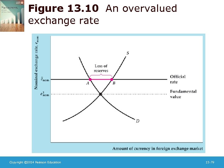
Figure 13. 10 An overvalued exchange rate Copyright © 2014 Pearson Education 13 -79

Fixed Exchange Rates • Fixing the exchange rate (Fig. 13. 11) – When the official rate is above its fundamental value, the currency is said to be overvalued – The country could devalue the currency, reducing the official rate to the fundamental value Copyright © 2014 Pearson Education 13 -80

Fixed Exchange Rates • Fixing the exchange rate (Fig. 13. 11) – The country could restrict international transactions to reduce the supply of its currency to the foreign exchange market, thus raising the fundamental value of the exchange rate – If a country prohibits people from trading the currency at all, the currency is said to be inconvertible Copyright © 2014 Pearson Education 13 -81

Fixed Exchange Rates • Fixing the exchange rate (Fig. 13. 11) – The government can supply or demand the currency to make the fundamental value equal to the official rate • If the currency is overvalued, the government can buy its own currency – This is done by the nation’s central bank using its official reserve assets to buy the domestic currency in the foreign exchange market – Official reserve assets include gold, foreign bank deposits, and special assets created by agencies like the International Monetary Fund – The decline in official reserve assets is equal to a country’s balance of payments deficit Copyright © 2014 Pearson Education 13 -82
Fixed Exchange Rates • Fixing the exchange rate – A country can’t maintain an overvalued currency forever, as it will run out of official reserve assets • In the gold standard period, countries sometimes ran out of gold and had to devalue their currencies Copyright © 2014 Pearson Education 13 -83

Fixed Exchange Rates • Fixing the exchange rate – A country can’t maintain an overvalued currency forever, as it will run out of official reserve assets • A speculative run (or speculative attack) may end the attempt to support an overvalued currency (Fig. 13. 12) – If investors think a currency may soon be devalued, they may sell assets denominated in the overvalued currency, increasing the supply of that currency on the foreign exchange market – This causes even bigger losses of official reserves from the central bank and speeds up the likelihood of devaluation, as occurred in Mexico in 1994 and Asia in 1997– 1998 • Thus an overvalued currency can’t be maintained for very long Copyright © 2014 Pearson Education 13 -84

Figure 13. 11 A speculative run on an overvalued currency Copyright © 2014 Pearson Education 13 -85
Fixed Exchange Rates • Fixing the exchange rate – Similarly, in the case of an undervalued currency, the official rate is below the fundamental value (Fig. 13) • In this case, a central bank trying to maintain the official rate will acquire official reserve assets • If the domestic central bank is gaining official reserve assets, foreign central banks must be losing them, so again the undervalued currency can’t be maintained for long Copyright © 2014 Pearson Education 13 -86
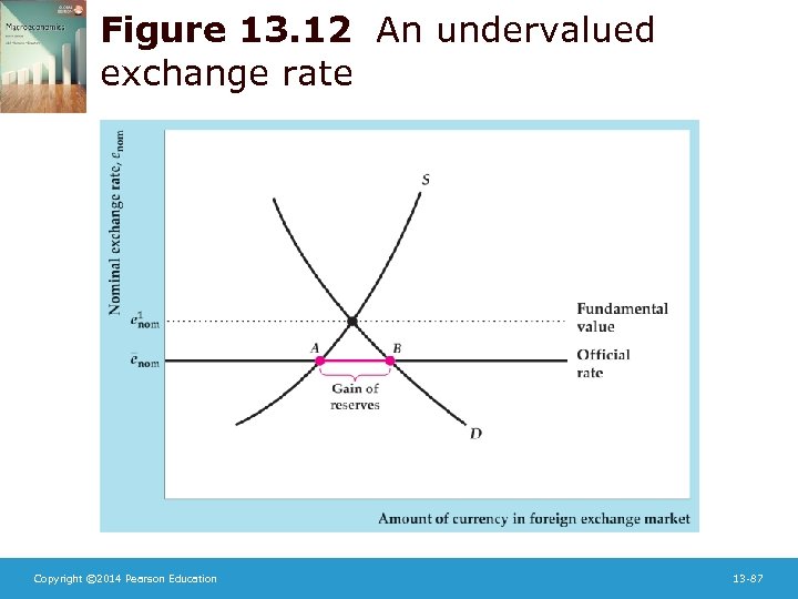
Figure 13. 12 An undervalued exchange rate Copyright © 2014 Pearson Education 13 -87
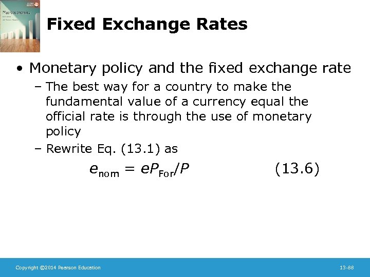
Fixed Exchange Rates • Monetary policy and the fixed exchange rate – The best way for a country to make the fundamental value of a currency equal the official rate is through the use of monetary policy – Rewrite Eq. (13. 1) as enom = e. PFor/P Copyright © 2014 Pearson Education (13. 6) 13 -88

Fixed Exchange Rates • Monetary policy and the fixed exchange rate – For an overvalued currency, a monetary contraction is desirable • In a Keynesian model, a monetary contraction causes a real (and nominal) exchange rate appreciation in the short run and a nominal exchange rate appreciation in the long run (with no long-run effect on the real exchange rate) • Conversely, a monetary expansion causes a nominal exchange rate depreciation in both the short run and the long run Copyright © 2014 Pearson Education 13 -89
Fixed Exchange Rates • Monetary policy and the fixed exchange rate – For an overvalued currency, a monetary contraction is desirable • Plotting the relationship between the money supply and the nominal exchange rate shows the level of the money supply for which the fundamental value of the exchange rate equals the official rate (Fig. 13. 14) Copyright © 2014 Pearson Education 13 -90

Figure 13. 13 Determination of the money supply under fixed exchange rates Copyright © 2014 Pearson Education 13 -91

Fixed Exchange Rates • Monetary policy and the fixed exchange rate – A higher money supply (than the level of the money supply for which the fundamental value of the exchange rate equals the official rate) yields an overvalued currency – A lower money supply yields an undervalued currency Copyright © 2014 Pearson Education 13 -92

Fixed Exchange Rates • Monetary policy and the fixed exchange rate – This implies that countries can’t both maintain the exchange rate and use monetary policy to affect output • Using expansionary monetary policy to fight a recession would lead to an overvalued currency • So under fixed exchange rates, monetary policy can’t be used for macroeconomic stabilization Copyright © 2014 Pearson Education 13 -93
Fixed Exchange Rates • Monetary policy and the fixed exchange rate – However, a group of countries may be able to coordinate their use of monetary policy • If two countries increase their money supplies together to fight joint recessions, there needn’t be an overvaluation • One country increasing its money supply by itself would lead to a depreciation • But when the other country increases its money supply, it provides an offsetting effect • If the money supplies expand in each country, they offset each other, so the exchange rate needn’t change (Fig. 13. 15) Copyright © 2014 Pearson Education 13 -94

Figure 13. 14 Coordinated monetary expansion Copyright © 2014 Pearson Education 13 -95
Fixed Exchange Rates • Monetary policy and the fixed exchange rate – Overall, fixed exchange rates can work well if countries in the system have similar macroeconomic goals and can coordinate changes in monetary policy • But the failure to cooperate can lead to severe problems Copyright © 2014 Pearson Education 13 -96
Fixed Exchange Rates • Fixed versus flexible exchange rates – Flexible-exchange-rate systems also have problems, because the volatility of exchange rates introduces uncertainty into international transactions – There are two major benefits of fixed exchange rates • Stable exchange rates make international trades easier and less costly • Fixed exchange rates help discipline monetary policy, making it impossible for a country to engage in expansionary policy; the result may be lower inflation in the long run Copyright © 2014 Pearson Education 13 -97

Fixed Exchange Rates • Fixed versus flexible exchange rates – But there are some disadvantages to fixed exchange rates • They take away a country’s ability to use expansionary monetary policy to combat recessions • Disagreement among countries about the conduct of monetary policy may lead to the breakdown of the system Copyright © 2014 Pearson Education 13 -98
Fixed Exchange Rates • Fixed versus flexible exchange rates – Which system is better may thus depend on the circumstances • If large benefits can be gained from increased trade and integration, and when countries can coordinate their monetary policies closely, then fixed exchange rates may be desirable • Countries that value having independent monetary policies, either because they face different macroeconomic shocks or hold different views about the costs of unemployment and inflation than other countries, should have a floating exchange rate Copyright © 2014 Pearson Education 13 -99
Fixed Exchange Rates • Currency unions – Under a currency union, countries agree to share a common currency • They often cooperate economically and politically as well, as was the case with the 13 original U. S. colonies Copyright © 2014 Pearson Education 13 -100

Fixed Exchange Rates • Currency unions – To work effectively, a currency union must have just one central bank • Since countries don’t usually want to give up control over monetary policy by not having their own central banks, currency unions are very rare • Advantages of currency unions over fixed exchange rates: reduces the costs of trading goods and assets across countries and because speculative attacks on a national currency can no longer occur Copyright © 2014 Pearson Education 13 -101
Fixed Exchange Rates • Currency unions – Major disadvantage: all countries share a common monetary policy, a problem that also arises with fixed exchange rates • Thus if one country is in recession while another is concerned about inflation, monetary policy can’t help both, whereas with flexible exchange rates, the countries could have monetary policies that help their particular situation Copyright © 2014 Pearson Education 13 -102
Fixed Exchange Rates • Application: European monetary unification – In 1991, countries in the European Community adopted the Maastricht treaty, which provides for a common currency • The currency, called the euro, came into being on January 1, 1999 • Eleven countries took part in the union, initially – Monetary policy is determined by the Governing Council of the European Central Bank (ECB) – The euro was introduced in 1999, but coins and currency were not issued until 2002 Copyright © 2014 Pearson Education 13 -103

Fixed Exchange Rates • Application: European monetary unification – The ECB differs from the Federal Reserve in two ways • In Europe, each individual country monitors its own banks, whereas in the United States, the Fed can set rules for all banks • In Europe, each country sets its own fiscal policy, whereas in the U. S. a central government determines fiscal policy Copyright © 2014 Pearson Education 13 -104

Fixed Exchange Rates • Application: European monetary unification – The U. S. and Europe differed in their handling of the financial crisis in 2008 • U. S. banks could raise capital more easily but European banks could not because each country regulated banks differently • Weakness at European banks cause the financial crisis to have a more prolonged effect on the European economy than the U. S. economy Copyright © 2014 Pearson Education 13 -105
Fixed Exchange Rates • Application: European monetary unification – European countries had violated the requirement to keep their government budget deficits low prior to the crisis • In the crisis, the countries lent to their banks, which increased the government budget deficit, which caused interest rates to rise, which caused banks to weaken further • So the government budget crisis in Europe is related to the financial crisis Copyright © 2014 Pearson Education 13 -106

Fixed Exchange Rates • Application: European monetary unification – Because of the euro, exchange rates between countries in good financial condition, such as Germany, and countries in weaker financial condition, such as Greece, could not adjust to restore equilibrium Copyright © 2014 Pearson Education 13 -107

Fixed Exchange Rates • Application: European monetary unification – The future of Europe is not clear • Countries such as Greece might drop out of the system • The system might be modified to keep countries from cheating on their budget deficits • Countries might give up some control over their banks and fiscal policies Copyright © 2014 Pearson Education 13 -108

Fixed Exchange Rates • Application: crisis in Argentina – Argentina’s economy has suffered periodic crises – Argentina’s inflation rate in the 1970 s and 1980 s was very large, with prices rising by a factor of 10 billion from 1975 to 1990 Copyright © 2014 Pearson Education 13 -109

Fixed Exchange Rates • Application: crisis in Argentina – Inflation was reduced to near zero in the 1990 s as the budget deficit was reduced and a currency board was implemented • A currency board is a monetary arrangement under which the supply of domestic currency in circulation is strictly limited by the amount of foreign reserves held by the central bank • A currency board works by limiting the money supply, ensuring low inflation • Argentina’s peso was backed one-for-one with U. S. dollars, and the exchange rate was fixed at one peso per dollar Copyright © 2014 Pearson Education 13 -110

Fixed Exchange Rates • Application: crisis in Argentina – The 1990 s were a time of economic prosperity for Argentina, with fast economic growth and low inflation – But the end of the decade saw Argentina slip into deep recession and the government’s budget deficit increased sharply • Argentina’s real exchange rate was overvalued in comparison with trading partners such as Brazil • Argentina ran large current account deficits in the 1990 s, and its foreign debt grew to about one-half of one year’s GDP Copyright © 2014 Pearson Education 13 -111

Fixed Exchange Rates • Application: crisis in Argentina – Eventually, Argentina defaulted on foreign debts and in January 2002 it abandoned the currency board, allowing the peso to float relative to the dollar • By July 2003, the peso was worth just $0. 36 • But the reduced real exchange rate allowed the economy to recover • Unfortunately, the inflation rate returned to double digits (averaging 11% per year from 2002 to 2011), so ultimately the currency board failed to deliver longterm price stability Copyright © 2014 Pearson Education 13 -112
a1c01335255533d0c7c8b4cbe49bee62.ppt