chapter: 12 > > Krugman/Wells Economics ©

chapter: 12 > > Krugman/Wells Economics © 2009 Worth Publishers. Behind the Supply Curve: Inputs and Costs

WHAT YOU WILL LEARN IN THIS CHAPTER The importance of the firm’s production function , the relationship between quantity of inputs and quantity of output Why production is often subject to diminishing returns to inputs The various types of costs a firm faces and how they generate the firm’s marginal and average cost curves Why a firm’s costs may differ in the short run versus the long run How the firm’s technology of production can generate increasing returns to scale

The Production Function A production function is the relationship between the quantity of inputs a firm uses and the quantity of output it produces. A fixed input is an input whose quantity is fixed for a period of time and cannot be varied. A variable input is an input whose quantity the firm can vary at any time.

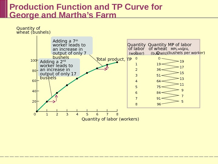
Inputs and Output The long run is the time period in which all inputs can be varied. The short run is the time period in which at least one input is fixed. The total product curve shows how the quantity of output depends on the quantity of the variable input, for a given quantity of the fixed input.

Production Function and TP Curve for George and Martha’s Farm 0 1 2 3 4 5 6 7 8 19 17 15 13 11 9 7 50 19 36 51 64 75 84 91 96 Quantity of labor L (worker) Quantity of wheat Q (bushels) MP of labor MPL = Q / L (bushels per worker) 7 86543210100 80 60 40 20 Quantity of wheat (bushels) Quantity of labor (workers) Total product, TPAdding a 7 th worker leads to an increase in output of only 7 bushels Adding a 2 nd worker leads to an increase in output of only 17 bushels

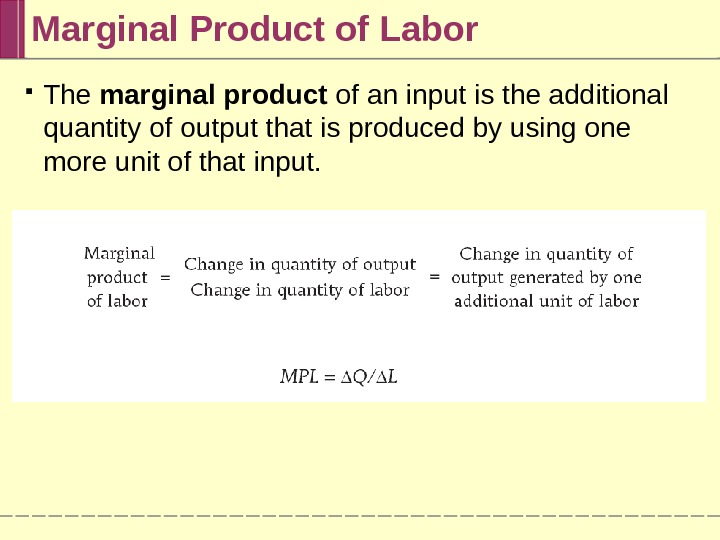
The marginal product of an input is the additional quantity of output that is produced by using one more unit of that input. Marginal Product of Labor

Diminishing Returns to an Input There are diminishing returns to an input when an increase in the quantity of that input, holding the levels of all other inputs fixed, leads to a decline in the marginal product of that input.

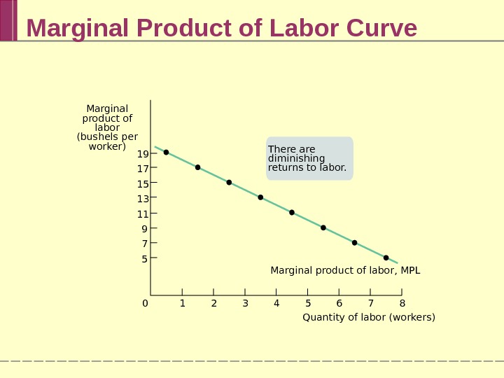
Marginal Product of Labor Curve Marginal product of labor, MPL 7 8654321019 17 15 13 11 9 7 5 Marginal product of labor (bushels per worker) Quantity of labor (workers)There are diminishing returns to labor.

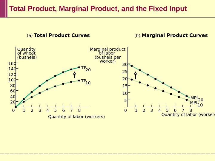
(a) Total Product Curves (b) Marginal Product Curves Marginal product of labor (bushels per worker)Quantity of wheat (bushels) 7 8654321030 25 20 15 10 5 7 86543210160 140 120 100 80 60 40 20 TP 10 MPL 20 MPL 10 Quantity of labor (workers)Total Product, Marginal Product, and the Fixed Input

From the Production Function to Cost Curves A fixed cost is a cost that does not depend on the quantity of output produced. It is the cost of the fixed input. A variable cost is a cost that depends on the quantity of output produced. It is the cost of the variable input.

Total Cost Curve The total cost of producing a given quantity of output is the sum of the fixed cost and the variable cost of producing that quantity of output. TC = FC + VC The total cost curve becomes steeper as more output is produced due to diminishing returns.

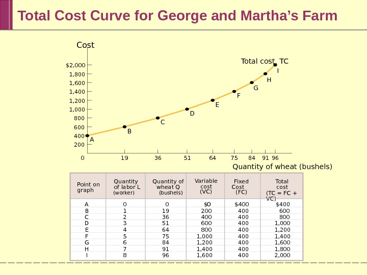
Total Cost Curve for George and Martha’s Farm 19 36 51 64 75 84 91 960$2, 000 1, 800 1, 600 1, 400 1, 200 1, 000 800 600 400 200 Cost Quantity of wheat (bushels)A B C D E F GTotal cost, TC H I A B C D E F G H IPoint on graph 0 1 2 3 4 5 6 7 8 $400 400 400 O 200 400 600 800 1, 000 1, 200 1, 400 1, 600 1, 800 2, 0000 19 36 51 64 75 84 91 96 Variable cost (VC) Total cost (TC = FC + VC) $ $Quantity of labor L (worker) Quantity of wheat Q (bushels) Fixed Cost (FC)

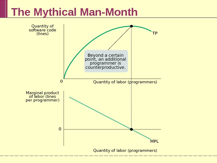
The Mythical Man-Month Quantity of labor (programmers) TP MPL 0 0 Quantity of labor (programmers)Marginal product of labor (lines per programmer) Quantity of software code (lines) Beyond a certain point, an additional programmer is counterproductive.

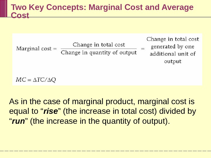
Two Key Concepts: Marginal Cost and Average Cost As in the case of marginal product, marginal cost is equal to “ rise ” (the increase in total cost) divided by “ run ” (the increase in the quantity of output).

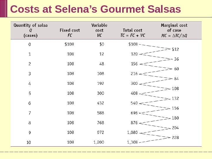
Costs at Selena’s Gourmet Salsas

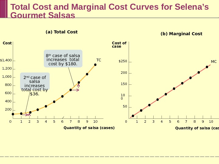
Total Cost and Marginal Cost Curves for Selena’s Gourmet Salsas $250 200 150 10 0 50 Cost of case 7 8 9 106543210 $1, 400 1, 200 1, 000 800 600 400 200 Cost Quantity of salsa (cases) 7 8 9 106543210 (b) Marginal Cost(a) Total Cost T C MC Quantity of salsa (cases)8 th case of salsa increases total cost by $180. 2 nd case of salsa increases total cost by $36.

Why is the Marginal Cost Curve Upward Sloping? Because there are diminishing returns to inputs in this example. As output increases, the marginal product of the variable input declines. This implies that more and more of the variable input must be used to produce each additional unit of output as the amount of output already produced rises. And since each unit of the variable input must be paid for, the cost per additional unit of output also rises.

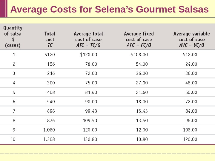
Average Cost Average total cost , often referred to simply as average cost , is total cost divided by quantity of output produced. ATC = TC/Q = (Total Cost) / (Quantity of Output) A U-shaped average total cost curve falls at low levels of output, then rises at higher levels. Average fixed cost is the fixed cost per unit of output. AFC = FC/Q = (Fixed Cost) / (Quantity of Output)

Average Cost Average variable cost is the variable cost per unit of output. AVC = VC/Q= (Variable Cost) / (Quantity of Output)

Average Total Cost Curve Increasing output has two opposing effects on average total cost: The spreading effect : the larger the output, the greater the quantity of output over which fixed cost is spread, leading to lower the average fixed cost. The diminishing returns effect : the larger the output, the greater the amount of variable input required to produce additional units leading to higher average variable cost.

Average Costs for Selena’s Gourmet Salsas

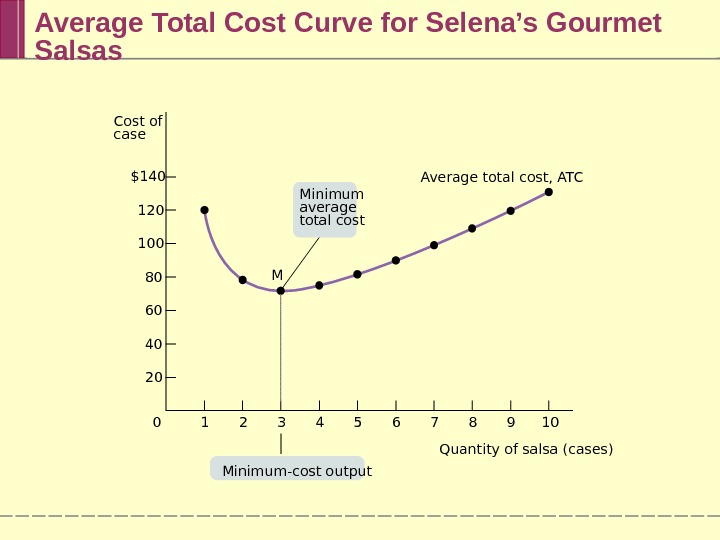
Average Total Cost Curve for Selena’s Gourmet Salsas Average total cost, ATC M 7 8 9 106543210$140 120 100 80 60 40 20 Minimum average total cost Minimum-cost output. Cost of case Quantity of salsa (cases)

Putting the Four Cost Curves Together Note that: 1. Marginal cost is upward sloping due to diminishing returns. 2. Average variable cost also is upward sloping but is flatter than the marginal cost curve. 3. Average fixed cost is downward sloping because of the spreading effect. 4. The marginal cost curve intersects the average total cost curve from below, crossing it at its lowest point. This last feature is our next subject of study.

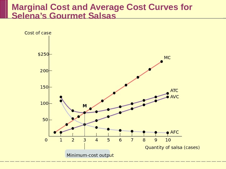
Marginal Cost and Average Cost Curves for Selena’s Gourmet Salsas $250 200 150 100 50 7 8 9 10654321 M 0 MC A T C A VC AFC Minimum-cost output. Cost of case Quantity of salsa (cases)

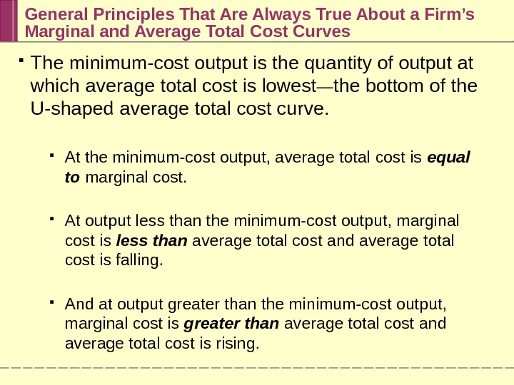
General Principles That Are Always True About a Firm’s Marginal and Average Total Cost Curves The minimum-cost output is the quantity of output at which average total cost is lowest — the bottom of the U-shaped average total cost curve. At the minimum-cost output, average total cost is equal to marginal cost. At output less than the minimum-cost output, marginal cost is less than average total cost and average total cost is falling. And at output greater than the minimum-cost output, marginal cost is greater than average total cost and average total cost is rising.

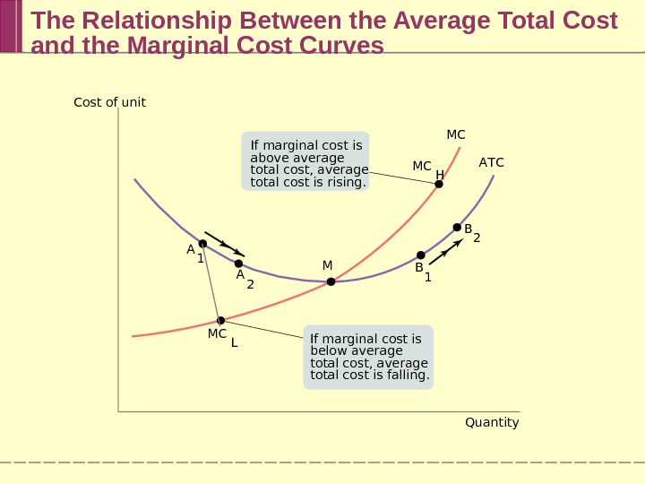
The Relationship Between the Average Total Cost and the Marginal Cost Curves Cost of unit Quantity. MC A T C MC L MC H A 1 B 1 A 2 B 2 MIf marginal cost is above average total cost, average total cost is rising. If marginal cost is below average total cost, average total cost is falling.

Does the Marginal Cost Curve Always Slope Upward? In practice, marginal cost curves often slope downward as a firm increases its production from zero up to some low level, sloping upward only at higher levels of production. This initial downward slope occurs because a firm that employs only a few workers often cannot reap the benefits of specialization of labor. This specialization can lead to increasing returns at first, and so to a downward-sloping marginal cost curve. Once there are enough workers to permit specialization, however, diminishing returns set in.

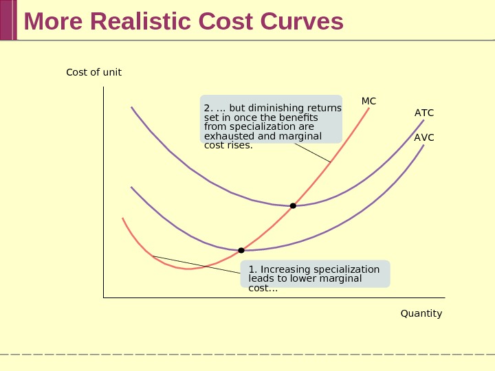
More Realistic Cost Curves MC A T C A VCCost of unit Quantity 2. … but diminishing returns set in once the benefits from specialization are exhausted and marginal cost rises. 1. Increasing specialization leads to lower marginal cost…

Short-Run versus Long-Run Costs In the short run, fixed cost is completely outside the control of a firm. But all inputs are variable in the long run. The firm will choose its fixed cost in the long run based on the level of output it expects to produce.

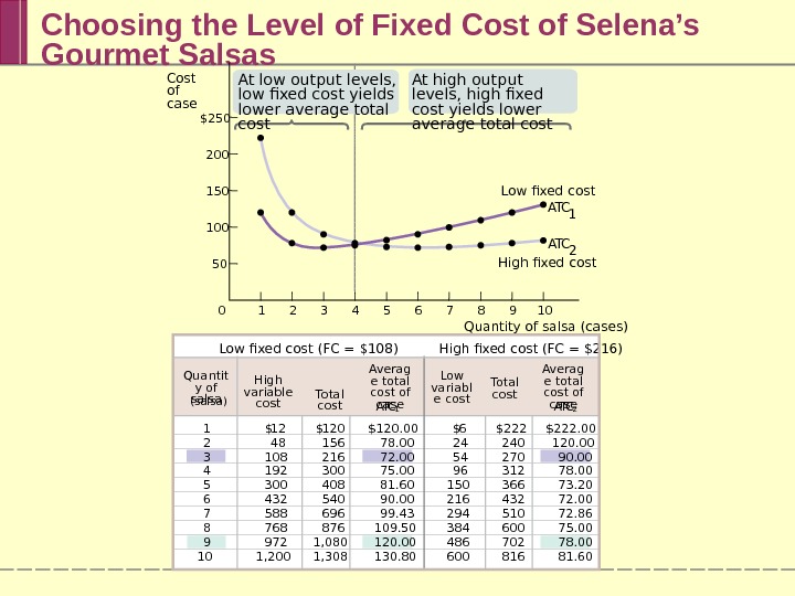
Choosing the Level of Fixed Cost of Selena’s Gourmet Salsas A T C 1 12 48 108 192 300 432 588 768 972 1, 200 $ 120 156 216 300 408 540 696 876 1, 080 1, 308 Total cost $ A T C 2 6 24 54 96 150 216 294 384 486 600 $ $222 240 270 312 366 432 510 600 702 816 Low fixed cost (FC = $108) High fixed cost (FC = $216) $120. 00 78. 00 72. 00 75. 00 81. 60 90. 00 99. 43 109. 50 120. 00 130. 80 $222. 00 120. 00 90. 00 78. 00 73. 20 72. 00 72. 86 75. 00 78. 00 81. 601 2 3 4 5 6 7 8 9 10 Averag e total cost of case. Quantit y of salsa (salsa) High variable cost Low variabl e cost Total cost Averag e total cost of case$250 200 150 100 50 Cost of case Quantity of salsa (cases)7 8 9 106543210 High fixed cost Low fixed cost A T C 2 A T C 1 At low output levels, low fixed cost yields lower average total cost At high output levels, high fixed cost yields lower average total cost

The long-run average total cost curve shows the relationship between output and average total cost when fixed cost has been chosen to minimize average total cost for each level of output. The Long-run Average Total Cost Curve

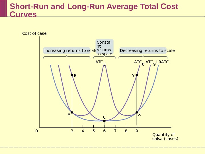
Short-Run and Long-Run Average Total Cost Curves B A T C 6 A T C 9 A T C 3 L R A T C 3 5 84 70 6 9 Increasing returns to scale Decreasing returns to scale. Consta nt returns to scale C XA YCost of case Quantity of salsa (cases)

Returns to Scale There are increasing returns to scale (economies of scale) when long-run average total cost declines as output increases. There are decreasing returns to scale ( diseconomies of scale) when long-run average total cost increases as output increases. There are constant returns to scale when long-run average total cost is constant as output increases.

SUMMARY 1. The relationship between inputs and output is a producer’s production function. In the short run , the quantity of a fixed input cannot be varied but the quantity of a variable input can. In the long run , the quantities of all inputs can be varied. For a given amount of the fixed input, the tota l product curve shows how the quantity of output changes as the quantity of the variable input changes. 2. There are diminishing returns to an input when its marginal product declines as more of the input is used, holding the quantity of all other inputs fixed. 3. Total cost is equal to the sum of fixed cost , which does not depend on output, and variable cost , which does depend on output.

SUMMARY 4. Average total cost , total cost divided by quantity of output, is the cost of the average unit of output, and marginal cost is the cost of one more unit produced. U-shaped average total cost curves are typical, because average total cost consists of two parts: average fixed cost , which falls when output increases (the spreading effect), and average variable cost , which rises with output (the diminishing returns effect). 5. When average total cost is U-shaped, the bottom of the U is the level of output at which average total cost is minimized, the point of minimum-cost output. This is also the point at which the marginal cost curve crosses the average total cost curve from below.

SUMMARY 6. In the long run, a producer can change its fixed input and its level of fixed cost. The long-run average total cost curve shows the relationship between output and average total cost when fixed cost has been chosen to minimize average total cost at each level of output. 7. As output increases, there are increasing returns to scale if long-run average total cost declines; decreasing returns to scale if it increases; and constant returns to scale if it remains constant. Scale effects depend on the technology of production.