Chapter 12 Basic option theory Investment Science D

Chapter 12: Basic option theory Investment Science D. G. Luenberger

Before we talk about options l l This course so far has dealt with deterministic cash flows and single-period random cash flows. Now we’d like to deal with random flows at each of several time points, i. e. , multiple random cash flows. Multiple random cash flow theories are generally very difficult. Here, we’d like to focus on a special case: derivatives, i. e. , those assets whose cash flows are functionally related to other assets whose price characteristics are assumed to be known. Options are an important category of derivatives.

Option, I l l An option is the right, but not the obligation, to buy (or sell) an underlying asset under specified terms. Usually there a specified price, called strike price or exercise price (K), and a specified period of time, called maturity (T) or expiration date, over which the option is valid. An option is a derivative because whose cash flows are related to the cash flows of the underlying asset. If the option holder actually does buy and sell the underlying asset, the option holder is said to exercise the option. The market price of an option is called premium.

Option, II l l An option that gives the right to purchase (sell) the underlying asset is called a call (put) option. An American option allows exercise at any time before and including the expiration date. An European option allows exercise only on the expiration date. In this course, we will focus on European options because their pricing is easier. The underlying assets of options can be financial securities, such as IBM shares or S&P 100 Index, or physical assets, such as wheat or corn.

Option, III l l l Many options are traded on open markets. Thus, their premiums are established in the market and observable. Options are wonderful instruments for managing business and investment risk, i. e. , hedging. Options can be particularly speculative because of their built-in leverages. For example, if you are very sure that IBM’s share price will go up, betting $1 on IBM call options may generate a much higher return than betting $1 on IBM shares.

Notation l l l S: the price of the underlying asset. C: the value of the call option. P: the value of the put option.

Value of call option at expiration

Value of put option at expiration

Value of option at expiration l l The value of the call at expiration: C = max (0, S – K). The call option is in the money, at the money, or out of money, depending on whether S > K, S = K, or S < K, respectively. The value of the put at expiration: P = max (0, K – S). The put option is in the money, at the money, or out of money, depending on whether S < K, S = K, or S > K, respectively.

11. 1 Binomial model, PP. 297 -299 l l A binomial model can be a single-period model or a multiple-period model. A basic period length can be a week, a month, a year, etc. If the price of an asset is known at the beginning of a period, say S, the price of the asst at the end of the period is one of only two possible values, S*u and S*d, where u > 1 > d > 0. S*u (S*d) is expected to happen with probability p (1 – p). That is, we have uncertainty, but in the form of two possible values.

Binomial model

Calibration, I l l Binomial models provide an uncertain structure for us to model the underlying asset’s price dynamics. This modeling is necessary because option value is a function of the underlying asset’s price dynamics. Thus, to obtain accurate valuation for an option, we need to do a good job on modeling the underlying asset’s price dynamics. That is, we need to choose binomial parameters, i. e. , p, u, and d, carefully such that the binomial-based price dynamics is consistent with the observable (historical) price characteristics, e. g. , average return and standard deviation, of the underlying asset.

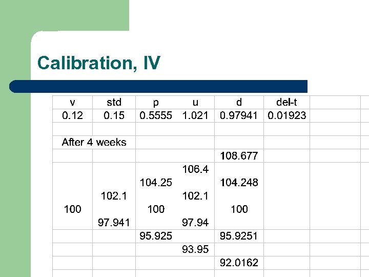
Calibration, II l l Let v be the expected (average) annual return of the underlying asset, v = E [ln(ST /S 0 )], say 12%. Let be the yearly standard deviation of the underlying asset, 2 = var [ln(ST /S 0 )], say 15%. Note that 12% return and 15% standard deviation are about the kind of numbers that you would expect from a typical S&P 500 stock. Now we need to define the period length relative to a year. If we define a period as a week, a period length of t is 1/52.

Calibration, III l l l Then, the binomial parameters can be selected as: p = ½ + ½ *(v / )* ( t)1/2. u = e * ( t)1/2. d = 1/u. e is exponential and has a value of 2. 7183. With these choices, the binomial model will closely match the values of v and (see pp. 313 -315 for the proof).

Calibration, IV

1 -period binomial option theory, I l l We assume that it is possible to borrow or lend at the risk-free rate, r. Let R = 1 + r, and u > R > d. Suppose that there is a call option on the underlying asset with strike price K and expiration at the end of the single period. Let Cu (Cd) be the value of the call at expiration.

3 related lattices

No-arbitrage l l The key to price the call option at time 0 is to form a portfolio at time 0: (1) the portfolio consists of the underlying asset and the risk-free asset, (2) the portfolio’s value at time 1 is equal to the value of the call at time 1, regardless whether it is up or down. This portfolio is called a replicating portfolio: x dollar worth of the underlying asset and b dollar worth of the risk-free asset. No-arbitrage: because the replicating portfolio and the call yield the value at time 1 regardless what might happen, the value of the replicating portfolio and the call at time 0 must be the same. That is, x + b = C.

Outcome matching l l l The value of the replicating portfolio equals to the value of the call at time 1 when it is up: u * x + R * b = C u. The value of the replicating portfolio equals to the value of the call at time 1 when it is down: d * x + R * b = C d. Solve for x and b from the two equations.

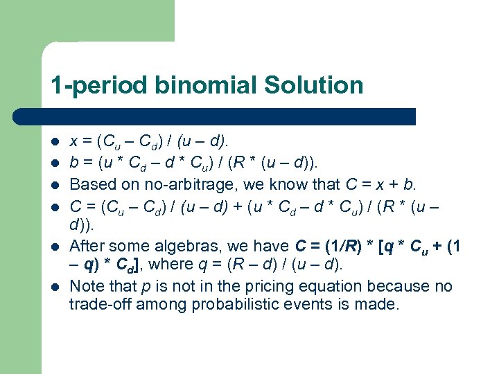
1 -period binomial Solution l l l x = (Cu – Cd) / (u – d). b = (u * Cd – d * Cu) / (R * (u – d)). Based on no-arbitrage, we know that C = x + b. C = (Cu – Cd) / (u – d) + (u * Cd – d * Cu) / (R * (u – d)). After some algebras, we have C = (1/R) * [q * Cu + (1 – q) * Cd], where q = (R – d) / (u – d). Note that p is not in the pricing equation because no trade-off among probabilistic events is made.

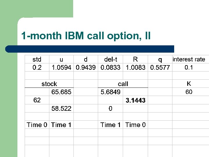
1 -month IBM call option, I l Consider IBM with a volatility of its logarithm of = 20%. The current price of IBM is $62. A call option on IBM has an expiration date 1 month from now and a strike price of $60. The current interest rate is 10%, compounded monthly. Suppose that IBM will not pay dividends.

1 -month IBM call option, II

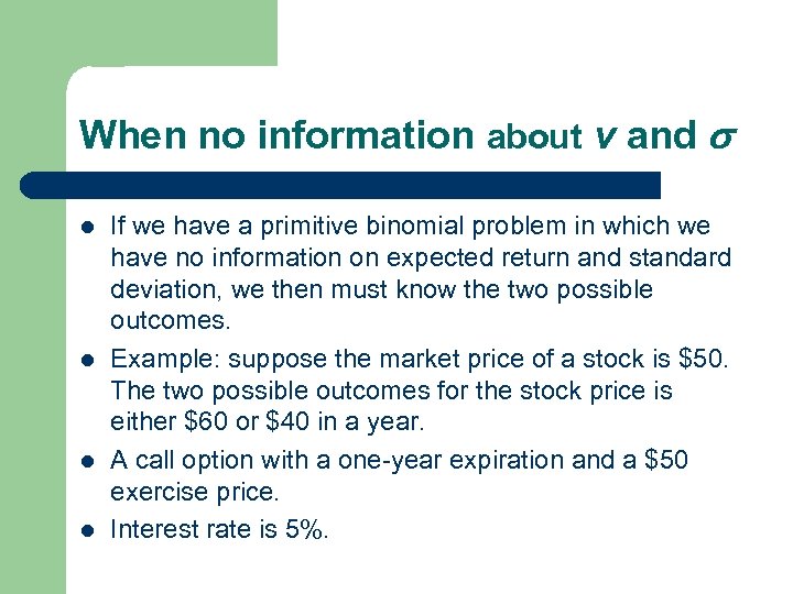
When no information about v and l l If we have a primitive binomial problem in which we have no information on expected return and standard deviation, we then must know the two possible outcomes. Example: suppose the market price of a stock is $50. The two possible outcomes for the stock price is either $60 or $40 in a year. A call option with a one-year expiration and a $50 exercise price. Interest rate is 5%.

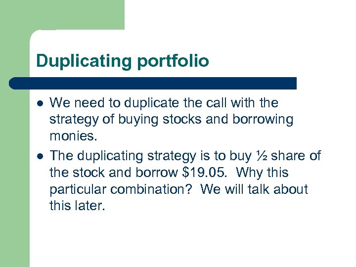
Duplicating portfolio l l We need to duplicate the call with the strategy of buying stocks and borrowing monies. The duplicating strategy is to buy ½ share of the stock and borrow $19. 05. Why this particular combination? We will talk about this later.

When the stock price is up l l When the stock price is up, the payoff of buying a call is $10 ($60 - $50). When the stock price is up, the payoff the duplicating strategy is also $10. The sum of the following two positions is $10 ($30 - $20): (1) buying ½ share: ½ * $60 = $30, and (2) borrowing $19. 05 at 5%: -$19. 05 * 1. 05 = $20.

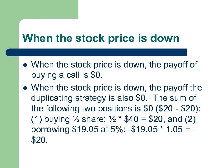
When the stock price is down l l When the stock price is down, the payoff of buying a call is $0. When the stock price is down, the payoff the duplicating strategy is also $0. The sum of the following two positions is $0 ($20 - $20): (1) buying ½ share: ½ * $40 = $20, and (2) borrowing $19. 05 at 5%: -$19. 05 * 1. 05 = $20.

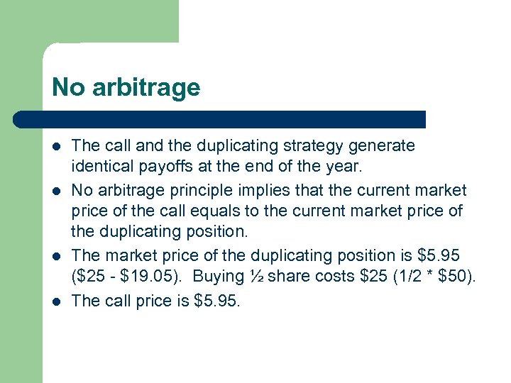
No arbitrage l l The call and the duplicating strategy generate identical payoffs at the end of the year. No arbitrage principle implies that the current market price of the call equals to the current market price of the duplicating position. The market price of the duplicating position is $5. 95 ($25 - $19. 05). Buying ½ share costs $25 (1/2 * $50). The call price is $5. 95.

Why ½ share? l l l The duplicating portfolio was given to be buying ½ share and borrowing $19. 05 earlier. Why ½ share? This amount is called the delta of the call. Delta = swing of the call / swing of the stock = ($10 - $0) / ($60 - $40) = ½.

Why borrowing $19. 05? l l l Buying ½ share gives us either $30 or $20 at expiration, which is exactly $20 higher than the payoffs of the call, $10 and $0, respectively. To duplicate the position, we thus need to borrow a dollar amount such that we will need to pay back exactly $20. Given the future value is $20, the interest rate is 5%, and the number of the time period is 1, we have the present value to be $19. 05 (use your financial calculator).

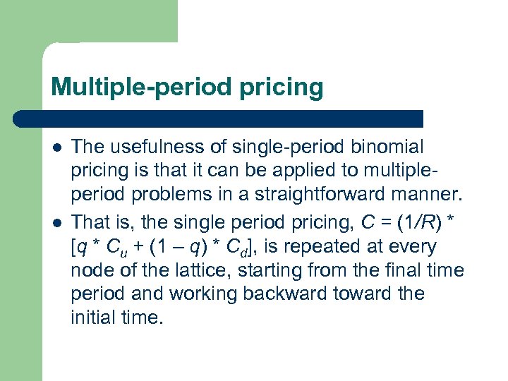
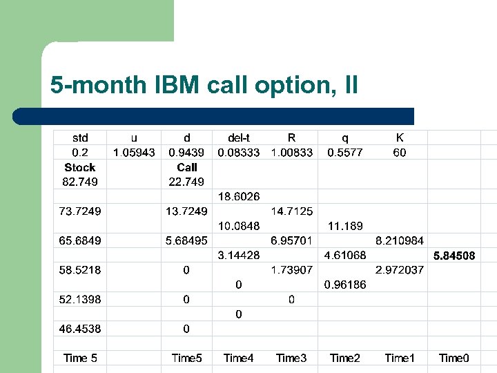
Multiple-period pricing l l The usefulness of single-period binomial pricing is that it can be applied to multipleperiod problems in a straightforward manner. That is, the single period pricing, C = (1/R) * [q * Cu + (1 – q) * Cd], is repeated at every node of the lattice, starting from the final time period and working backward toward the initial time.

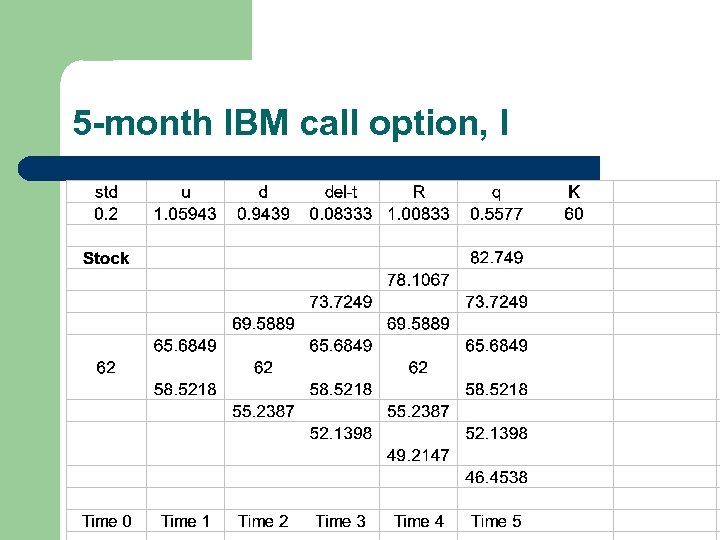
5 -month IBM call option, I

5 -month IBM call option, II

1 -month vs. 5 -month l l l The call price for 1 -month IBM call is $3. 14. The call price for 5 -month IBM call is $5. 85. Holding other factors constant, the longer the maturity, the higher the call premium. The reason for this is that additional time allows for a greater chance for the stock to rise in value, increasing the final payoff of the call option. See Figure 12. 3, p. 324. Along the same line of seasoning, the higher the standard deviation, the higher the call premium. You should verify this numerically.

How about put option pricing? l l So far, we have focused on call pricing. The reason for this is that for European options one can calculate the value of a put option, P, based on value the call option, C, when they have the same strike price and maturity. P = C – S + df * K, where df is risk-free discount factor. This relationship is called the put-call parity.

Put option pricing l l Consider a GM call option and a GM put option, both have 3 months to expiration and the same strike price, $35. The current price of GM shares is $37. 78. The call premium is $4. 25. The interest rate is 5. 5%, so over 3 months, the discount factor is 0. 986 (= 1 / (1 + 0. 055/4). P = C – S + df * K = 4. 25 – 37. 78 + 0. 986 * 35 = $1. 00.

Options are interesting and important l l A combination of options can lead to a unique payoff structure that otherwise would not be possible. Options make it happen! Example: a butterfly spread, p. 325. Question: who would hold a butterfly spread?