Chapter 12 Aggregate Demand Aggregate Supply Aggregate

Chapter 12 Aggregate Demand Aggregate Supply

Aggregate Demand Aggregate Supply -- used to explain short-run fluctuations in real GDP and price level Aggregate Demand -- Curve showing the quantity of real GDP demanded by households, firms and Gov’t at various price levels Short-Run Aggregate Supply (SRAS) -- Curve showing the quantity of real GDP supplied by firms at various price levels in short run

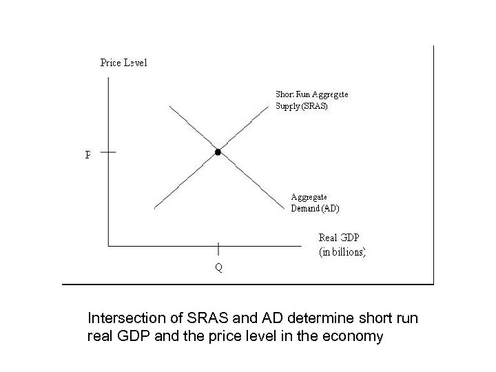Intersection of SRAS and AD determine short run real GDP and the price level in the economy

Derivation of Downward Slope -- as P ↓, quantity demanded of real GDP ↑ Effect of ∆P on C, I and Xn (G is unaffected by price level changes): 1) Wealth Effect (Influence on C) -- when the price level ↑, real value of wealth ↓ ↓ in consumption -- when the price level , real value of wealth ↑ ↑ in consumption

2) Interest Rate Effect (Influence on I and to a degree C) -- when price level ↑, households & businesses need more money to continue buying/selling. -- increase demand for money leads to increase in banking withdrawals, increase borrowing and/or selling of financial assets rise in interest rates on loans and bonds -- as r ↑, leads to less borrowing by firms for capital expenditures (new buildings, machinery, etc) and households will borrow less for new homes. Also consumption is affected with reduced purchases of durable goods

3) International Trade Effect -- if price level ↑ relative to other countries, U. S. exports become more expensive and imports become less expensive foreigners buy more domestic or non-U. S. goods and U. S. consumers purchase more foreign goods Decrease in exports and increase in imports Decrease in net exports -- reverse effect if price level ↓

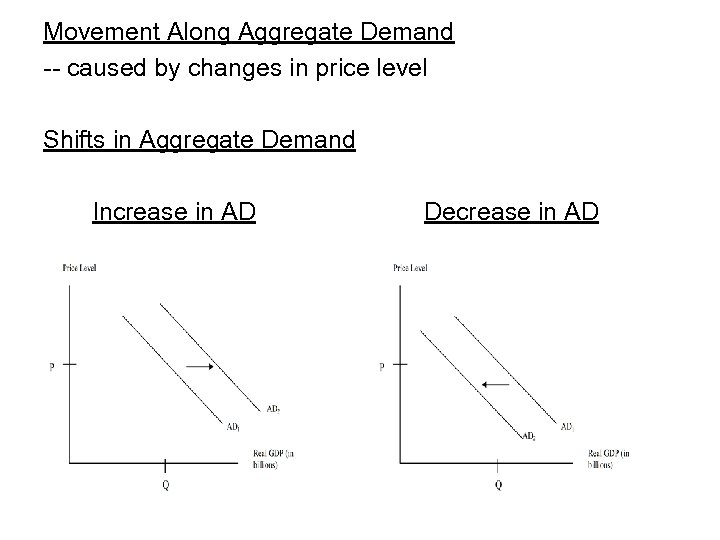Movement Along Aggregate Demand -- caused by changes in price level Shifts in Aggregate Demand Increase in AD Decrease in AD

Shifts in Aggregate Demand -- When variables other than price change 1) ∆ Government Policies -- Influence of Monetary Policy (∆ in interest rates) and Fiscal Policy (Gov’t purchases and taxes) a) As r ↑, cost of borrowing ↑ C and I ↓ AD shifts left As r ↓, cost of borrowing ↓ C and I ↑ shifts AD right b) As Gov’t purchases ↑ AD shifts right As Gov’t purchases ↓ AD shifts left c) As taxes↑ disposable income ↓ C ↓ shifts AD left As taxes ↓ disposable income ↑ C ↑ shifts AD right

2) ∆ Expectations of Firms/Households -- If households are more optimistic about future incomes C ↑ shifts AD right -- If households are more pessimistic C ↓ AD shifts left -- If firms become more optimistic about future payoff of investment spending AD shifts right -- If firms become more pessimistic AD shifts left 3) ∆ Foreign Variables -- If U. S. real GDP grows faster than real GDP in other countries increase in income for U. S. consumers is greater than that of foreign consumers Imports will increase faster than exports net exports ↓ AD shifts left (opposite occurs when real GDP grows at a slower pace relative to other countries) -- Net Exports ↓ when exchange rates between U. S. dollar and foreign currency ↑ (dollar increases in value) because prices in foreign countries for U. S. goods ↑ (reduces exports) while prices foreign goods in U. S. ↓ (increases imports) AD shift left (opposite occurs when exchange rates between U. S. and foreign currency ↓) Note: ∆ in net exports from change in price level does not shift AD

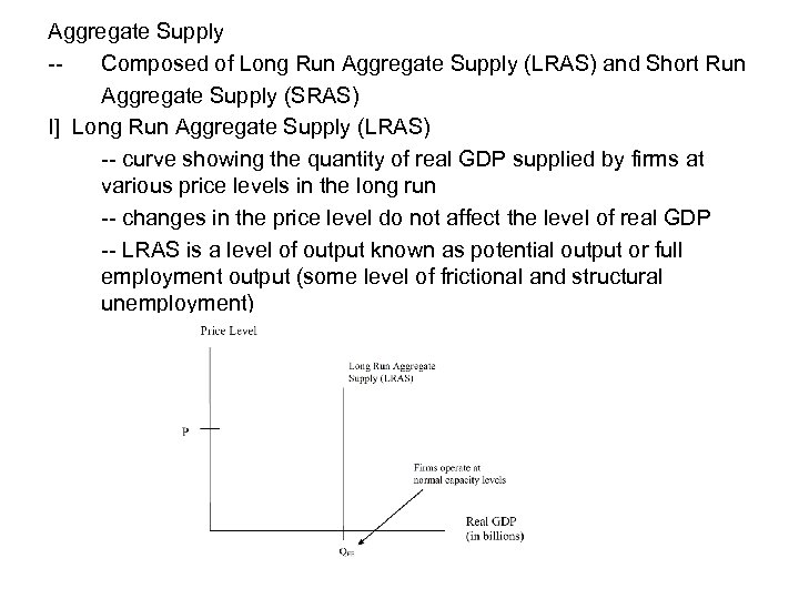Aggregate Supply -Composed of Long Run Aggregate Supply (LRAS) and Short Run Aggregate Supply (SRAS) I] Long Run Aggregate Supply (LRAS) -- curve showing the quantity of real GDP supplied by firms at various price levels in the long run -- changes in the price level do not affect the level of real GDP -- LRAS is a level of output known as potential output or full employment output (some level of frictional and structural unemployment)

I] Short Run Aggregate Supply (SRAS) -- upward sloping because as price ↑, quantity supplied of goods and services by firms ↑ Reasons for upward slope: 1) Increased Profits: Prices of inputs rise slower than price of goods/services hence greater profits 2) Firms are slow to adjust prices: -- As prices ↑, some firms are slow to increase their prices and therefore experience an increase in sales/increase in production. -- As prices ↓, some firms are slow to adjust their prices ↓ so they experience a reduction in sales/decrease in production

Reasons Behind Reasons i) Contracts make wages and prices “sticky” -- “sticky” refers to the fact that wages and prices are slow to react to changes in demand supply Example: #1) Company X and union negotiate a multi-year wage contract. The company’s sales begin to take off and therefore prices ↑ in the midst of stable wages leading to increased profits #2) Company X enters an agreement with a supplier to supply a key input at a constant price for 2 yrs. If sales take off and prices ↑, since price inputs remains constant, profits ↑ Note: Although examples reflect specific companies, pervasive scenarios can influence entire economy.

Reasons Behind Reasons ii) Firms adjust wages slowly -- Many non-union wage adjustments occur once a year when during the course of the year, prices can fluctuate considerably. Also, wages are often more conservatively adjusted after careful evaluation of the state of the economy, historical increases, and financial condition of the company. As a result, we say wages adjust slowly compared to price levels in the marketplace. iii) Menu costs make prices “sticky” -- Many firms have menus or catalogs that contain a list of their products’ prices. Prices are set after careful evaluation of market conditions and demand. -- As prices rise and fall, even though firms would want to change their prices, there would be associated costs with making any changes. These costs are known as menu costs (costs to firms of changing prices)

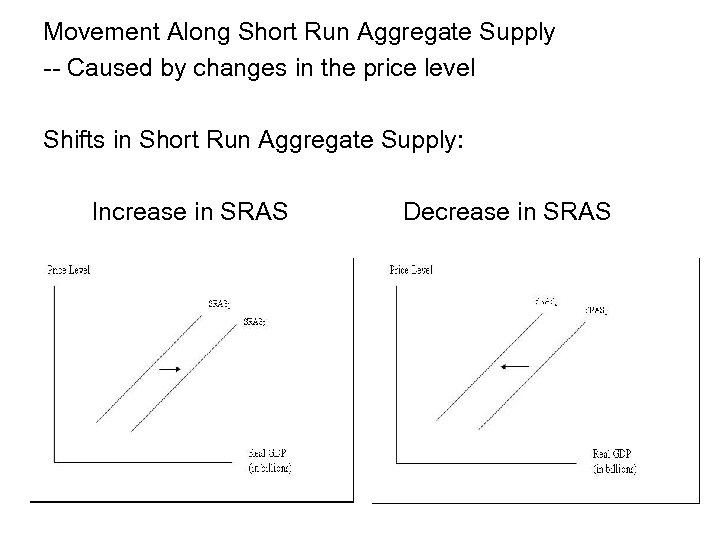Movement Along Short Run Aggregate Supply -- Caused by changes in the price level Shifts in Short Run Aggregate Supply: Increase in SRAS Decrease in SRAS

Shifts in Short Run Aggregate Supply: -- When variables other than price change 1) Increase in Labor Force and in Capital Stock -- firms will increase output at every price level if the # workers increase or capital increase SRAS shifts to the right (more output can be produced at every price level) 2) Technological Change -- with technological change, productivity of workers and machines increase, meaning firms can increase output w/o any adjustment in amount of labor and capital reduction in units costs and greater profitability as output increases SRAS shifts to the right

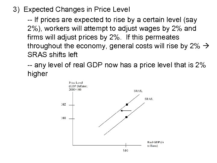3) Expected Changes in Price Level -- If prices are expected to rise by a certain level (say 2%), workers will attempt to adjust wages by 2% and firms will adjust prices by 2%. If this permeates throughout the economy, general costs will rise by 2% SRAS shifts left -- any level of real GDP now has a price level that is 2% higher

4) Adjustment of Workers and Firms to Errors in Past Expectations About Price Levels -- If workers and firms make inaccurate predictions about the price level, they will attempt to make it up in the future (price and wage adjustments) a) If, economy-wide, price level was higher than expected (planned and set prices @ lower price point), firms adjust prices ↑ & workers’ wages ↑ SRAS shifts left. b) If, economy-wide, price level was lower than expected (planned and set prices @ higher price point), firms adjust prices ↓ & workers’ wages ↓ SRAS shifts right.

5) Unexpected Changes in Price of Critical Natural Resource -- Unexpected increases/decreases in critical natural resources can cause firms’ costs to change. There are some natural resources that can have an economy-wide effect (e. g. oil—can effect utility costs, transportation costs, raw material costs, etc, depending on industry of firm) -- Increase in cost of critical resource on output will cause SRAS to shift left while a decrease in cost of critical resource will cause SRAS to shift right. Spending Shock: Unexpected event causing SRAS to shift • Often the result of unexpected changes in a critical resource

Macroeconomic Equilibrium I] Short-Run Equilibrium: -- level of output where AD intersects SRAS -- Price level is in terms of GDP Deflator (could have chosen CPI) GDP Deflator = Nominal GDP X 100 Real GDP Example: GDP Deflator value of 106 tells us that prices were 6% higher than in base year

Macroeconomic Equilibrium II] Long Run Equilibrium: -level of output where AD = SRAS = LRAS -economy is at potential output or level of output @ full employment

Impact of Recessions, Expansions and Spending Shocks On Equilibrium Assumptions: 1) Economy is not experiencing inflation 2) Economy is not experiencing avg long run growth A) Recessions -- Households become pessimistic about future incomes and firms become pessimistic about future profitability of investments AD Shifts left

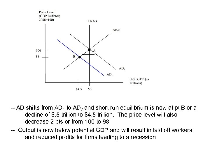-- AD shifts from AD 1 to AD 2 and short run equilibrium is now at pt B or a decline of $. 5 trillion to $4. 5 trillion. The price level will also decrease 2 pts or from 100 to 98 -- Output is now below potential GDP and will result in laid off workers and reduced profits for firms leading to a recession

Adjustment Back to Potential Output -- With drop in output, price level drops to 98. Workers and firms adjust to the price level being lower than expected by ↓ in wages (able to buy more and unemployed workers willing to accept lower wages to be able to work) and firms prices ↓ (firms accept lower price due to reduced demand) shifts SRAS to the right and over time back to full employment level (pt C). Price level decreases further to 96.

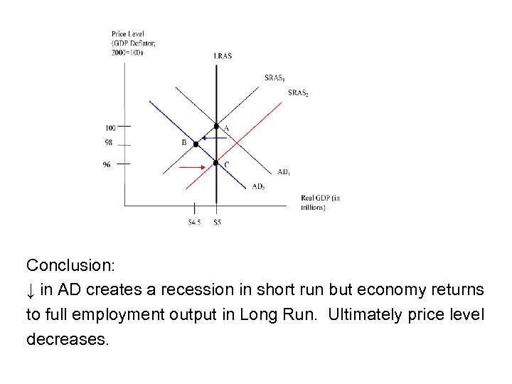Conclusion: ↓ in AD creates a recession in short run but economy returns to full employment output in Long Run. Ultimately price level decreases.

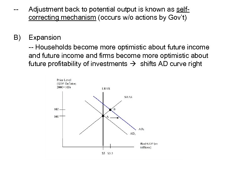-- Adjustment back to potential output is known as selfcorrecting mechanism (occurs w/o actions by Gov’t) B) Expansion -- Households become more optimistic about future income and firms become more optimistic about future profitability of investments shifts AD curve right

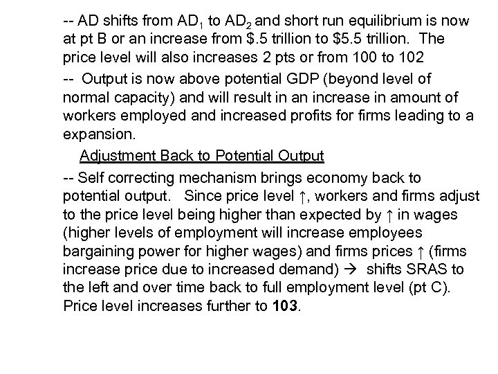-- AD shifts from AD 1 to AD 2 and short run equilibrium is now at pt B or an increase from $. 5 trillion to $5. 5 trillion. The price level will also increases 2 pts or from 100 to 102 -- Output is now above potential GDP (beyond level of normal capacity) and will result in an increase in amount of workers employed and increased profits for firms leading to a expansion. Adjustment Back to Potential Output -- Self correcting mechanism brings economy back to potential output. Since price level ↑, workers and firms adjust to the price level being higher than expected by ↑ in wages (higher levels of employment will increase employees bargaining power for higher wages) and firms prices ↑ (firms increase price due to increased demand) shifts SRAS to the left and over time back to full employment level (pt C). Price level increases further to 103.

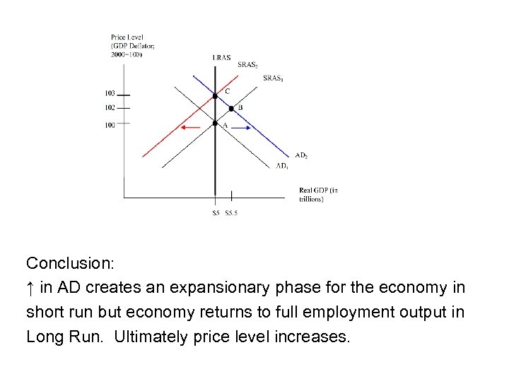Conclusion: ↑ in AD creates an expansionary phase for the economy in short run but economy returns to full employment output in Long Run. Ultimately price level increases.

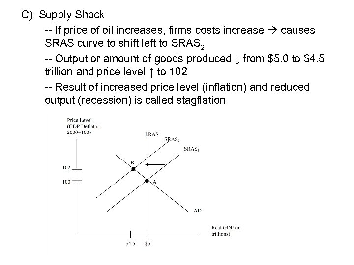C) Supply Shock -- If price of oil increases, firms costs increase causes SRAS curve to shift left to SRAS 2 -- Output or amount of goods produced ↓ from $5. 0 to $4. 5 trillion and price level ↑ to 102 -- Result of increased price level (inflation) and reduced output (recession) is called stagflation

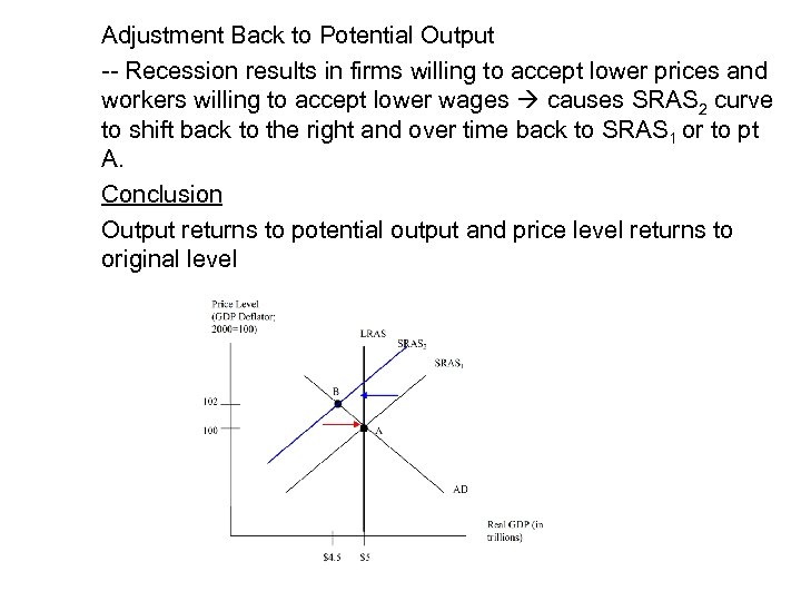Adjustment Back to Potential Output -- Recession results in firms willing to accept lower prices and workers willing to accept lower wages causes SRAS 2 curve to shift back to the right and over time back to SRAS 1 or to pt A. Conclusion Output returns to potential output and price level returns to original level