Chapter 11 Pricing with Market Power Chapter 11

Chapter 11 Pricing with Market Power Chapter 11 1

Topics to be Discussed n Capturing Consumer Surplus n Price Discrimination n Intertemporal Price Discrimination and Peak-Load Pricing Chapter 11 2

Topics to be Discussed n The Two-Part Tariff n Bundling n Advertising Chapter 11 3

Introduction n Pricing without market power (perfect competition) is determined by market supply and demand. n The individual producer must be able to forecast the market and then concentrate on managing production (cost) to maximize profits. Chapter 11 4

Introduction n Pricing with market power (imperfect competition) requires the individual producer to know much more about the characteristics of demand as well as manage production. Chapter 11 5

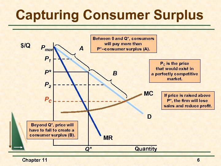Capturing Consumer Surplus $/Q Pmax Between 0 and Q*, consumers will pay more than P*--consumer surplus (A). A P 1 P* B P 2 PC is the price that would exist in a perfectly competitive market. MC PC If price is raised above P*, the firm will lose sales and reduce profit. D Beyond Q*, price will have to fall to create a consumer surplus (B). MR Q* Chapter 11 Quantity 6

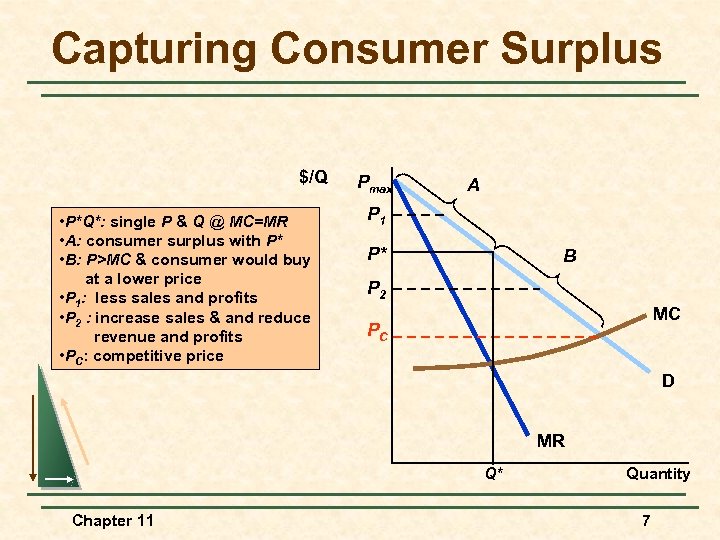Capturing Consumer Surplus $/Q • P*Q*: single P & Q @ MC=MR • A: consumer surplus with P* • B: P>MC & consumer would buy at a lower price • P 1: less sales and profits • P 2 : increase sales & and reduce revenue and profits • PC: competitive price Pmax A P 1 P* B P 2 MC PC D MR Q* Chapter 11 Quantity 7

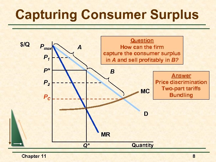Capturing Consumer Surplus $/Q Pmax Question How can the firm capture the consumer surplus in A and sell profitably in B? A P 1 P* B P 2 MC PC Answer Price discrimination Two-part tariffs Bundling D MR Q* Chapter 11 Quantity 8

Capturing Consumer Surplus n Price discrimination is the charging of different prices to different consumers for similar goods. Chapter 11 9

Price Discrimination n First Degree Price Discrimination l Chapter 11 Charge a separate price to each customer: the maximum or reservation price they are willing to pay. 10

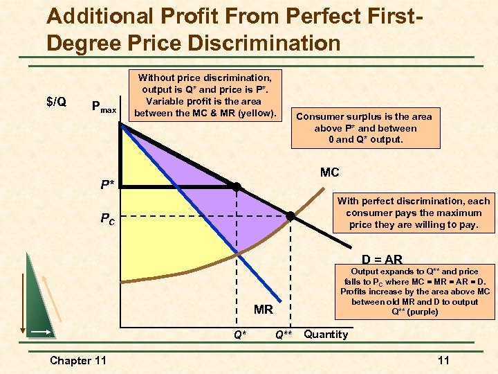Additional Profit From Perfect First. Degree Price Discrimination $/Q Pmax Without price discrimination, output is Q* and price is P*. Variable profit is the area between the MC & MR (yellow). Consumer surplus is the area above P* and between 0 and Q* output. MC P* With perfect discrimination, each consumer pays the maximum price they are willing to pay. PC D = AR Output expands to Q** and price falls to PC where MC = MR = AR = D. Profits increase by the area above MC between old MR and D to output Q** (purple) MR Q* Chapter 11 Q** Quantity 11

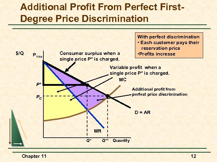Additional Profit From Perfect First. Degree Price Discrimination $/Q Pmax Consumer surplus when a single price P* is charged. With perfect discrimination • Each customer pays their reservation price • Profits increase Variable profit when a single price P* is charged. MC P* Additional profit from perfect price discrimination PC D = AR MR Q* Chapter 11 Q** Quantity 12

Additional Profit From Perfect First. Degree Price Discrimination n Question l n Why would a producer have difficulty in achieving first-degree price discrimination? Answer 1) Too many customers (impractical) 2) Could not estimate the reservation price for each customer Chapter 11 13

Price Discrimination n First Degree Price Discrimination l Chapter 11 The model does demonstrate the potential profit (incentive) of practicing price discrimination to some degree. 14

Price Discrimination n First Degree Price Discrimination l Examples of imperfect price discrimination where the seller has the ability to segregate the market to some extent and charge different prices for the same product: Lawyers, doctors, accountants u Car salesperson (15% profit margin) u Colleges and universities u Chapter 11 15

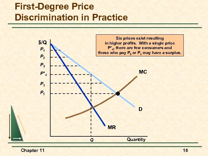First-Degree Price Discrimination in Practice Six prices exist resulting in higher profits. With a single price P*4, there are few consumers and those who pay P 5 or P 6 may have a surplus. $/Q P 1 P 2 P 3 MC P*4 P 5 P 6 D MR Q Chapter 11 Quantity 16

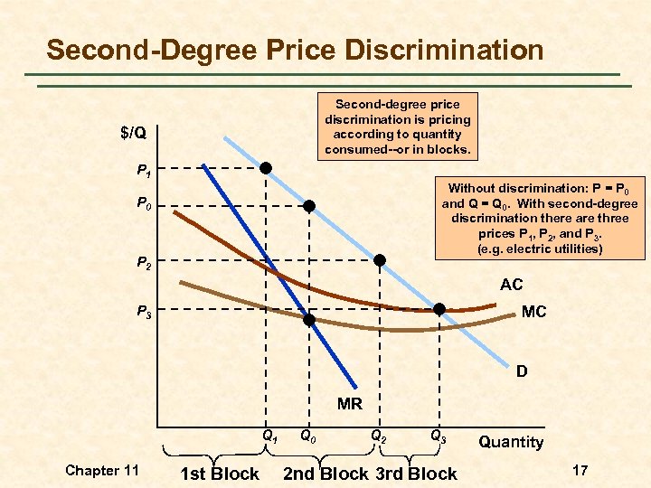Second-Degree Price Discrimination Second-degree price discrimination is pricing according to quantity consumed--or in blocks. $/Q P 1 Without discrimination: P = P 0 and Q = Q 0. With second-degree discrimination there are three prices P 1, P 2, and P 3. (e. g. electric utilities) P 0 P 2 AC P 3 MC D MR Q 1 Chapter 11 1 st Block Q 0 Q 2 Q 3 2 nd Block 3 rd Block Quantity 17

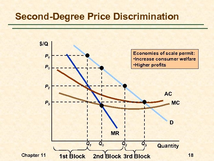Second-Degree Price Discrimination $/Q Economies of scale permit: • Increase consumer welfare • Higher profits P 1 P 0 P 2 AC P 3 MC D MR Q 1 Chapter 11 1 st Block Q 0 Q 2 Q 3 2 nd Block 3 rd Block Quantity 18

Price Discrimination n Third Degree Price Discrimination 1) Divides the market into two-groups. 2) Each group has its own demand function. Chapter 11 19

Price Discrimination n Third Degree Price Discrimination 3) Most common type of price discrimination. u Chapter 11 Examples: airlines, liquor, vegetables, discounts to students and senior citizens. 20

Price Discrimination n Third Degree Price Discrimination 4) Third-degree price discrimination is feasible when the seller can separate his/her market into groups who have different price elasticities of demand (e. g. business air travelers versus vacation air travelers) Chapter 11 21

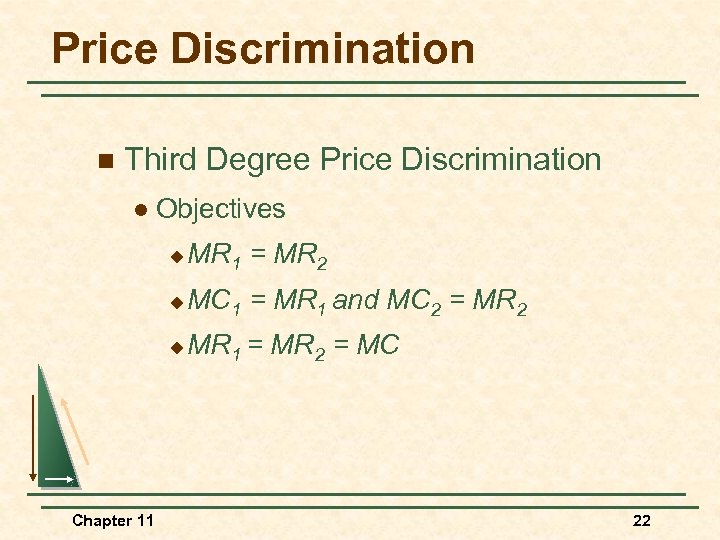Price Discrimination n Third Degree Price Discrimination l Objectives u u MC 1 = MR 1 and MC 2 = MR 2 u Chapter 11 MR 1 = MR 2 = MC 22

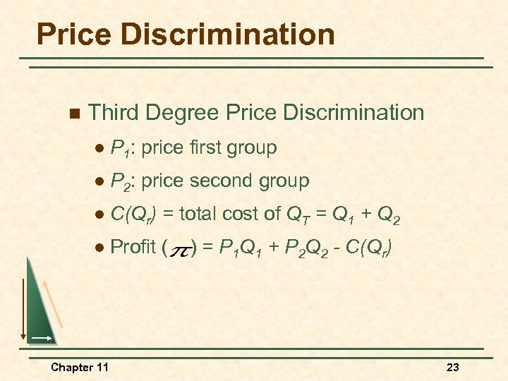Price Discrimination n Third Degree Price Discrimination l P 1: price first group l P 2: price second group l C(Qr) = total cost of QT = Q 1 + Q 2 l Profit ( Chapter 11 ) = P 1 Q 1 + P 2 Q 2 - C(Qr) 23

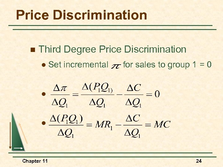Price Discrimination n Third Degree Price Discrimination l Set incremental for sales to group 1 = 0 l l Chapter 11 24

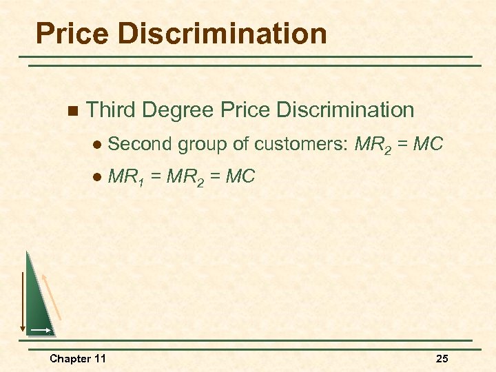Price Discrimination n Third Degree Price Discrimination l Second group of customers: MR 2 = MC l MR 1 = MR 2 = MC Chapter 11 25

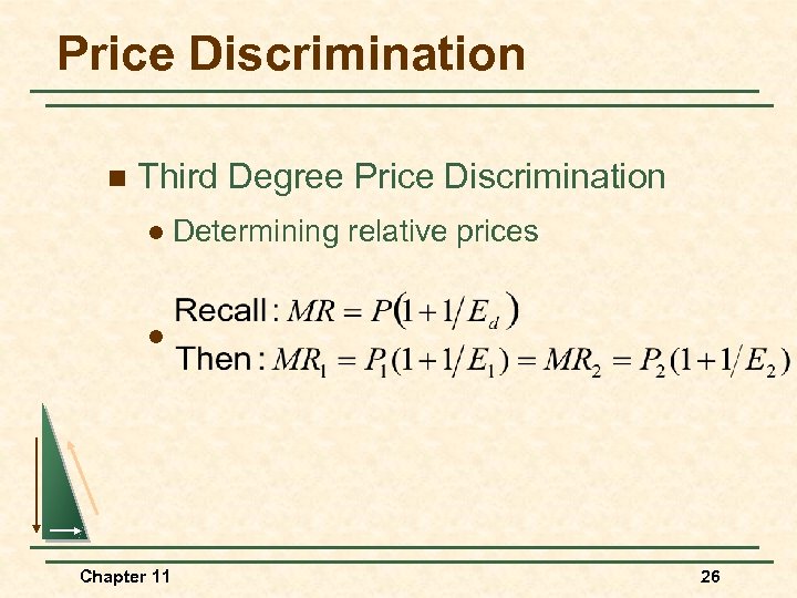Price Discrimination n Third Degree Price Discrimination l Determining relative prices l Chapter 11 26

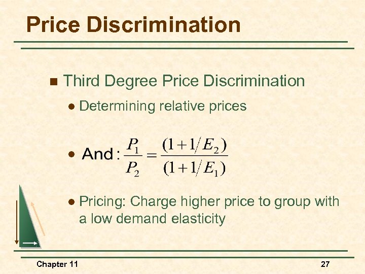Price Discrimination n Third Degree Price Discrimination l Determining relative prices l l Chapter 11 Pricing: Charge higher price to group with a low demand elasticity 27

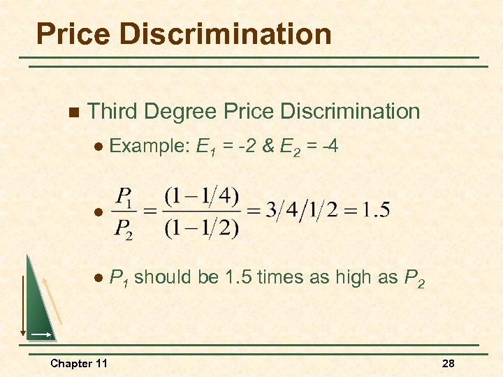Price Discrimination n Third Degree Price Discrimination l Example: E 1 = -2 & E 2 = -4 l l Chapter 11 P 1 should be 1. 5 times as high as P 2 28

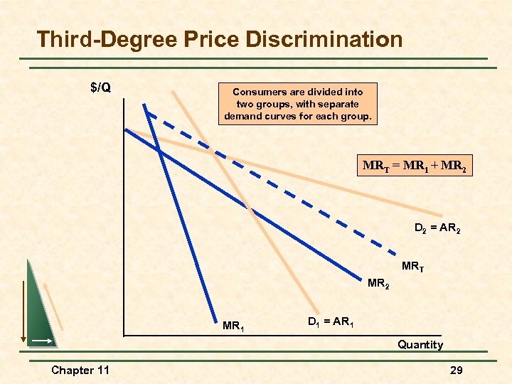Third-Degree Price Discrimination $/Q Consumers are divided into two groups, with separate demand curves for each group. MRT = MR 1 + MR 2 D 2 = AR 2 MRT MR 2 MR 1 D 1 = AR 1 Quantity Chapter 11 29

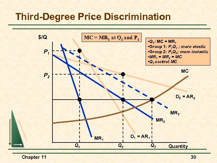Third-Degree Price Discrimination $/Q MC = MR 1 at Q 1 and P 1 • QT: MC = MRT • Group 1: P 1 Q 1 ; more elastic • Group 2: P 2 Q 2; more inelastic • MR 1 = MR 2 = MC • QT control MC MC P 2 D 2 = AR 2 MRT MR 2 D 1 = AR 1 MR 1 Q 1 Chapter 11 Q 2 QT Quantity 30

No Sales to Smaller Market Even if third-degree price discrimination is feasible, it doesn’t always pay to sell to both groups of consumers if marginal cost is rising. Chapter 11 31

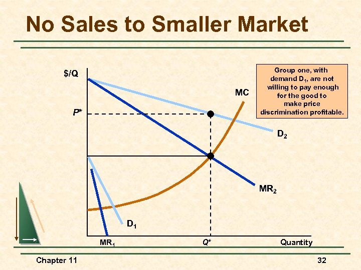No Sales to Smaller Market $/Q MC P* Group one, with demand D 1, are not willing to pay enough for the good to make price discrimination profitable. D 2 MR 2 D 1 MR 1 Chapter 11 Q* Quantity 32

The Economics of Coupons and Rebates Price Discrimination n Those consumers who are more price elastic will tend to use the coupon/rebate more often when they purchase the product than those consumers with a less elastic demand. n Coupons and rebate programs allow firms to price discriminate. Chapter 11 33

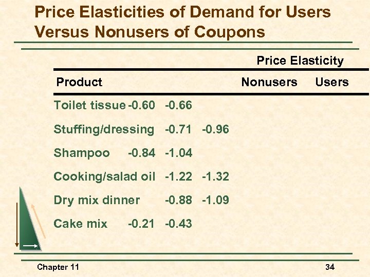Price Elasticities of Demand for Users Versus Nonusers of Coupons Price Elasticity Product Nonusers Users Toilet tissue -0. 60 -0. 66 Stuffing/dressing -0. 71 -0. 96 Shampoo -0. 84 -1. 04 Cooking/salad oil -1. 22 -1. 32 Dry mix dinner Cake mix Chapter 11 -0. 88 -1. 09 -0. 21 -0. 43 34

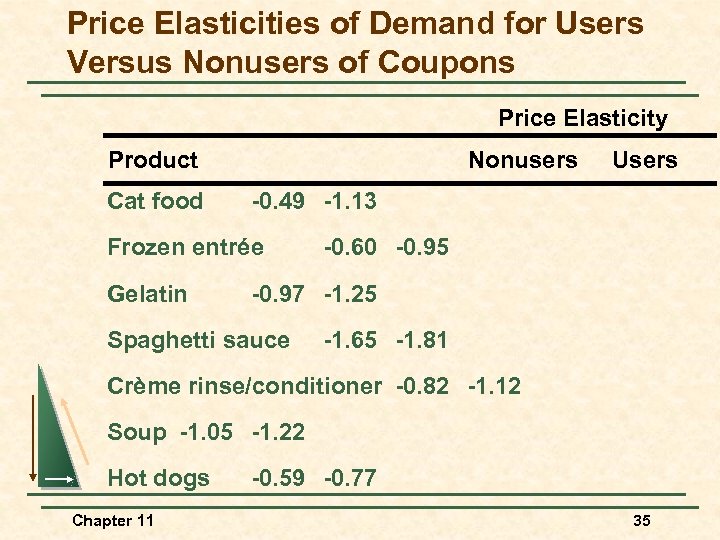Price Elasticities of Demand for Users Versus Nonusers of Coupons Price Elasticity Product Cat food Nonusers -0. 49 -1. 13 Frozen entrée Gelatin Users -0. 60 -0. 95 -0. 97 -1. 25 Spaghetti sauce -1. 65 -1. 81 Crème rinse/conditioner -0. 82 -1. 12 Soup -1. 05 -1. 22 Hot dogs Chapter 11 -0. 59 -0. 77 35

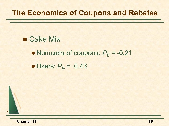The Economics of Coupons and Rebates n Cake Mix l Nonusers l Users: Chapter 11 of coupons: PE = -0. 21 PE = -0. 43 36

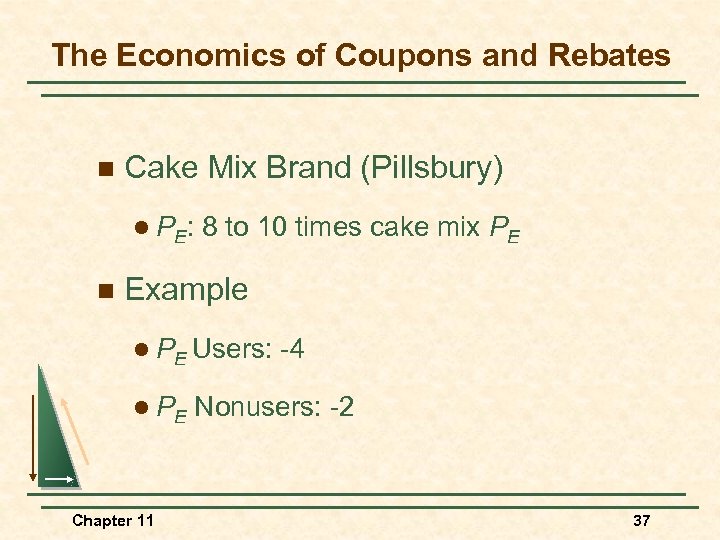The Economics of Coupons and Rebates n Cake Mix Brand (Pillsbury) l P E: n 8 to 10 times cake mix PE Example l PE Users: l PE Chapter 11 -4 Nonusers: -2 37

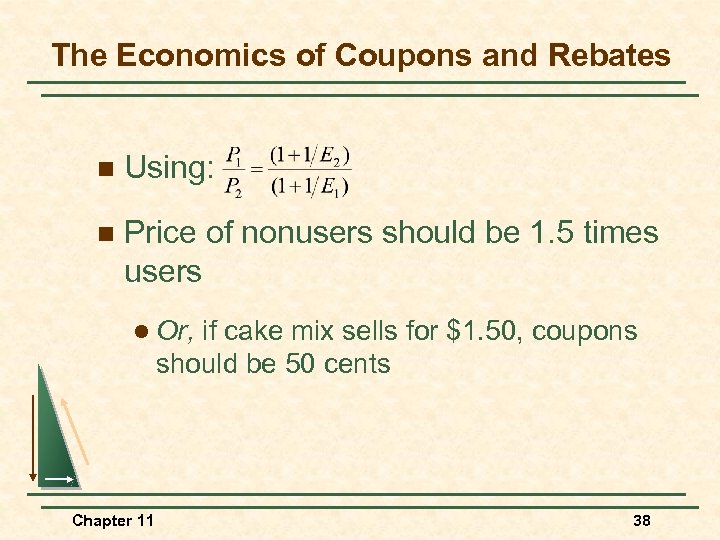The Economics of Coupons and Rebates n Using: n Price of nonusers should be 1. 5 times users l Or, if cake mix sells for $1. 50, coupons should be 50 cents Chapter 11 38

Airline Fares n Differences in elasticities imply that some customers will pay a higher fare than others. n Business travelers have few choices and their demand is less elastic. n Casual travelers have choices and are more price sensitive. Chapter 11 39

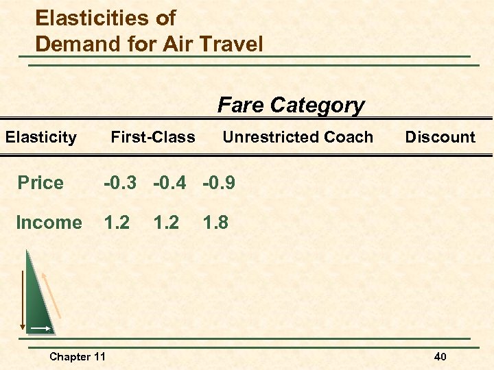Elasticities of Demand for Air Travel Fare Category Elasticity First-Class Unrestricted Coach Price -0. 3 -0. 4 -0. 9 Income 1. 2 Discount Chapter 11 1. 2 1. 8 40

Airline Fares n The airlines separate the market by setting various restrictions on the tickets. l Less expensive: notice, stay over the weekend, no refund l Most expensive: no restrictions Chapter 11 41

Intertemporal Price Discrimination and Peak-Load Pricing n Separating the Market With Time l Initial release of a product, the demand is inelastic u u Movie u Chapter 11 Book Computer 42

Intertemporal Price Discrimination and Peak-Load Pricing n Separating the Market With Time l Once this market has yielded a maximum profit, firms lower the price to appeal to a general market with a more elastic demand u u Dollar Movies u Chapter 11 Paper back books Discount computers 43

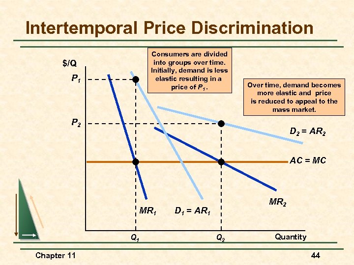Intertemporal Price Discrimination Consumers are divided into groups over time. Initially, demand is less elastic resulting in a price of P 1. $/Q P 1 Over time, demand becomes more elastic and price is reduced to appeal to the mass market. P 2 D 2 = AR 2 AC = MC MR 1 Q 1 Chapter 11 MR 2 D 1 = AR 1 Q 2 Quantity 44

Intertemporal Price Discrimination and Peak-Load Pricing n Demand for some products may peak at particular times. l Rush hour traffic l Electricity - late summer afternoons l Ski resorts on weekends Chapter 11 45

Intertemporal Price Discrimination and Peak-Load Pricing n Capacity restraints will also increase MC. n Increased MR and MC would indicate a higher price. Chapter 11 46

Intertemporal Price Discrimination and Peak-Load Pricing n MR is not equal for each market because one market does not impact the other market. Chapter 11 47

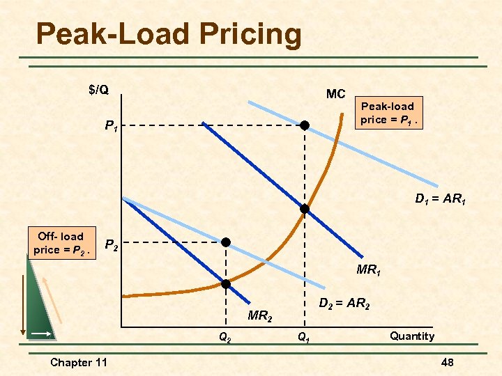Peak-Load Pricing $/Q MC P 1 Peak-load price = P 1. D 1 = AR 1 Off- load price = P 2 MR 1 D 2 = AR 2 MR 2 Q 2 Chapter 11 Q 1 Quantity 48

How to Price a Best Selling Novel n What Do You Think? 1) How would you arrive at the price for the initial release of the hardbound edition of a book? Chapter 11 49

How to Price a Best Selling Novel n What Do You Think? 2) How long do you wait to release the paperback edition? Could the popularity of the book impact your decision? Chapter 11 50

How to Price a Best Selling Novel n What Do You Think? 3) How do you determine the price for the paperback edition? Chapter 11 51

The Two-Part Tariff n The purchase of some products and services can be separated into two decisions, and therefore, two prices. Chapter 11 52

The Two-Part Tariff n Examples 1) Amusement Park Pay to enter u Pay for rides and food within the park u 2) Tennis Club Pay to join u Pay to play u Chapter 11 53

The Two-Part Tariff n Examples 3) Rental of Mainframe Computers Flat Fee u Processing Time u 4) Safety Razor Pay for razor u Pay for blades u Chapter 11 54

The Two-Part Tariff n Examples 5) Polaroid Film u u Chapter 11 Pay for the camera Pay for the film 55

The Two-Part Tariff n Pricing decision is setting the entry fee (T) and the usage fee (P). n Choosing the trade-off between freeentry and high use prices or high-entry and zero use prices. Chapter 11 56

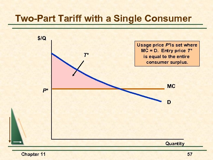Two-Part Tariff with a Single Consumer $/Q T* P* Usage price P*is set where MC = D. Entry price T* is equal to the entire consumer surplus. MC D Quantity Chapter 11 57

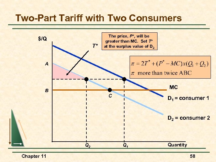Two-Part Tariff with Two Consumers $/Q T* The price, P*, will be greater than MC. Set T* at the surplus value of D 2. A MC B C D 1 = consumer 1 D 2 = consumer 2 Q 2 Chapter 11 Q 1 Quantity 58

The Two-Part Tariff n The Two-Part Tariff With Many Different Consumers l No exact way to determine P* and T*. l Must consider the trade-off between the entry fee T* and the use fee P*. u Chapter 11 Low entry fee: High sales and falling profit with lower price and more entrants. 59

The Two-Part Tariff n The Two-Part Tariff With Many Different Consumers l To find optimum combination, choose several combinations of P, T. l Choose the combination that maximizes profit. Chapter 11 60

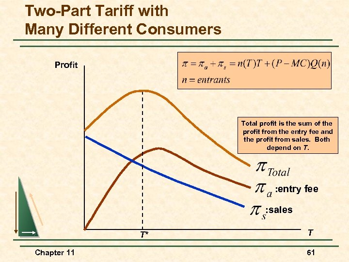Two-Part Tariff with Many Different Consumers Profit Total profit is the sum of the profit from the entry fee and the profit from sales. Both depend on T. : entry fee : sales T* Chapter 11 T 61

The Two-Part Tariff n Rule of Thumb l Similar demand: Choose P close to MC and high T l Dissimilar demand: Choose high P and low T. Chapter 11 62

The Two-Part Tariff n Two-Part Tariff With A Twist l Entry price (T) entitles the buyer to a certain number of free units u u Amusement parks with some tokens u Chapter 11 Gillette razors with several blades On-line with free time 63

Polaroid Cameras n 1971 Polaroid introduced the SX-70 camera n What Do You Think? l How Chapter 11 would you price the camera and film? 64

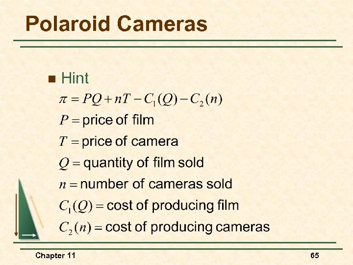Polaroid Cameras n Hint Chapter 11 65

Pricing Cellular Phone Service n Question l Why do cellular phone providers offer several different plans instead of a single two-part tariff with an access fee and perunit charge? Chapter 11 66

Bundling n Bundling is packaging two or more products to gain a pricing advantage. n Conditions necessary for bundling l Heterogeneous customers l Price discrimination is not possible l Demands must be negatively correlated Chapter 11 67

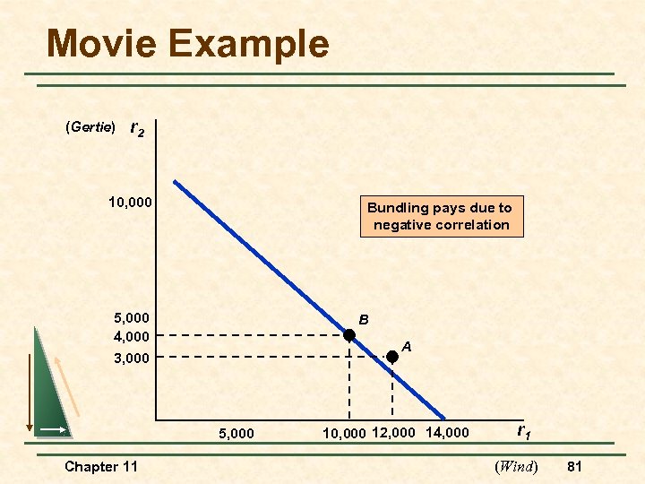
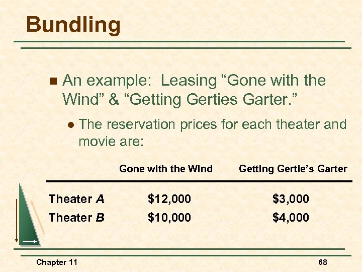Bundling n An example: Leasing “Gone with the Wind” & “Getting Gerties Garter. ” l The reservation prices for each theater and movie are: Gone with the Wind Getting Gertie’s Garter Theater A $12, 000 $3, 000 Theater B $10, 000 $4, 000 Chapter 11 68

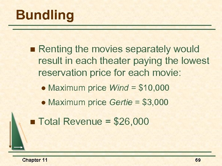Bundling n Renting the movies separately would result in each theater paying the lowest reservation price for each movie: l l n Maximum price Wind = $10, 000 Maximum price Gertie = $3, 000 Total Revenue = $26, 000 Chapter 11 69

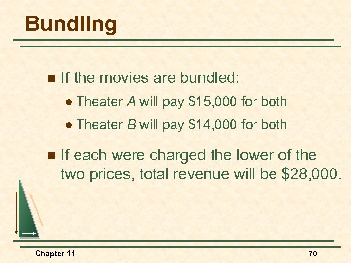Bundling n If the movies are bundled: l l n Theater A will pay $15, 000 for both Theater B will pay $14, 000 for both If each were charged the lower of the two prices, total revenue will be $28, 000. Chapter 11 70

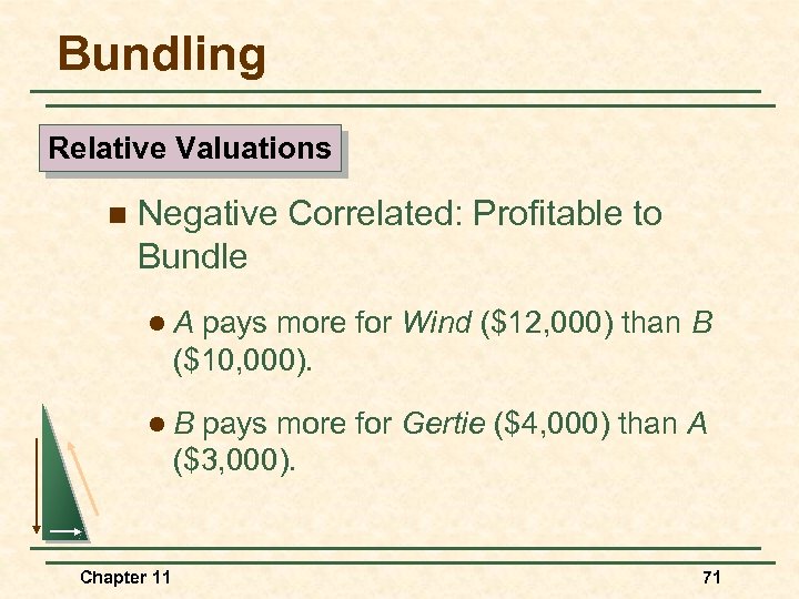Bundling Relative Valuations n Negative Correlated: Profitable to Bundle l. A pays more for Wind ($12, 000) than B ($10, 000). l. B pays more for Gertie ($4, 000) than A ($3, 000). Chapter 11 71

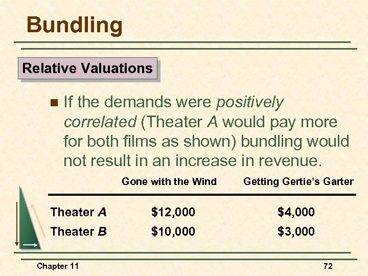Bundling Relative Valuations n If the demands were positively correlated (Theater A would pay more for both films as shown) bundling would not result in an increase in revenue. Gone with the Wind Getting Gertie’s Garter Theater A $12, 000 $4, 000 Theater B $10, 000 $3, 000 Chapter 11 72

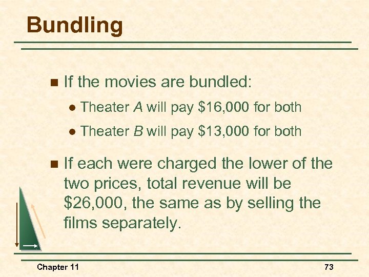Bundling n If the movies are bundled: l l n Theater A will pay $16, 000 for both Theater B will pay $13, 000 for both If each were charged the lower of the two prices, total revenue will be $26, 000, the same as by selling the films separately. Chapter 11 73

Bundling n Bundling Scenario: Two different goods and many consumers l Chapter 11 Many consumers with different reservation price combinations for two goods 74

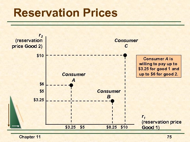Reservation Prices r 2 (reservation price Good 2) Consumer C $10 $6 Consumer A Consumer B $5 $3. 25 Chapter 11 Consumer A is willing to pay up to $3. 25 for good 1 and up to $6 for good 2. $5 $8. 25 $10 r 1 (reservation price Good 1) 75

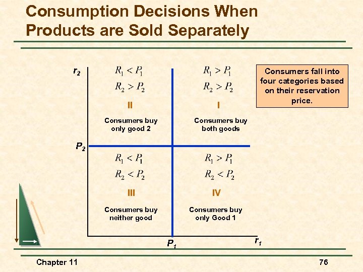Consumption Decisions When Products are Sold Separately r 2 II I Consumers buy only good 2 Consumers fall into four categories based on their reservation price. Consumers buy both goods P 2 III IV Consumers buy neither good Consumers buy only Good 1 P 1 Chapter 11 r 1 76

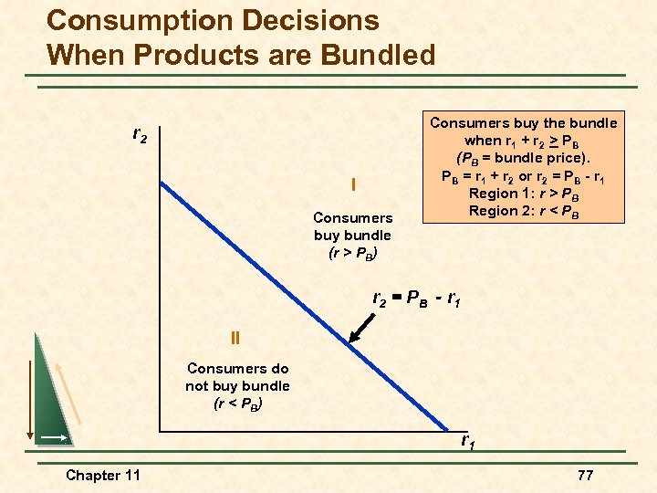Consumption Decisions When Products are Bundled r 2 I Consumers buy bundle (r > PB) Consumers buy the bundle when r 1 + r 2 > PB (PB = bundle price). PB = r 1 + r 2 or r 2 = PB - r 1 Region 1: r > PB Region 2: r < PB r 2 = P B - r 1 II Consumers do not buy bundle (r < PB) r 1 Chapter 11 77

Consumption Decisions When Products are Bundled n The effectiveness of bundling depends upon the degree of negative correlation between the two demands. Chapter 11 78

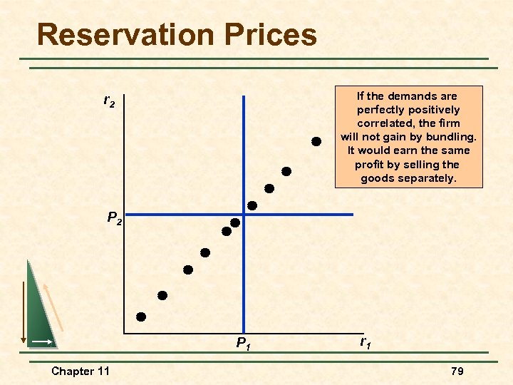Reservation Prices If the demands are perfectly positively correlated, the firm will not gain by bundling. It would earn the same profit by selling the goods separately. r 2 P 1 Chapter 11 r 1 79

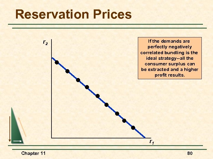Reservation Prices r 2 If the demands are perfectly negatively correlated bundling is the ideal strategy--all the consumer surplus can be extracted and a higher profit results. r 1 Chapter 11 80

Movie Example (Gertie) r 2 10, 000 Bundling pays due to negative correlation 5, 000 4, 000 3, 000 B A 5, 000 Chapter 11 10, 000 12, 000 14, 000 r 1 (Wind) 81

Bundling n Mixed Bundling l n Selling both as a bundle and separately Pure Bundling l Chapter 11 Selling only a package 82

Mixed Versus Pure Bundling r 2 100 C 1 = MC 1 = 20 A With positive marginal costs, mixed bundling may be more profitable than pure bundling. 90 80 70 60 50 40 B C Consumer A, for example, has a reservation price for good 1 that is below marginal cost c 1. With mixed bundling, consumer A is induced to buy only good 2, while consumer D is induced to buy only good 1, reducing the firm’s cost. 30 20 D C 2 = MC 2 = 30 10 10 20 30 40 50 60 70 80 90 100 Chapter 11 r 1 83

Bundling Mixed vs. Pure Bundling n Scenario l Perfect negative correlation l Significant marginal cost Chapter 11 84

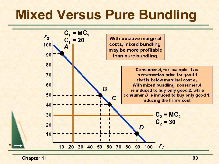
Bundling Mixed vs. Pure Bundling n Observations l Reservation price is below MC for some consumers l Mixed bundling induces the consumers to buy only goods for which their reservation price is greater than MC Chapter 11 85

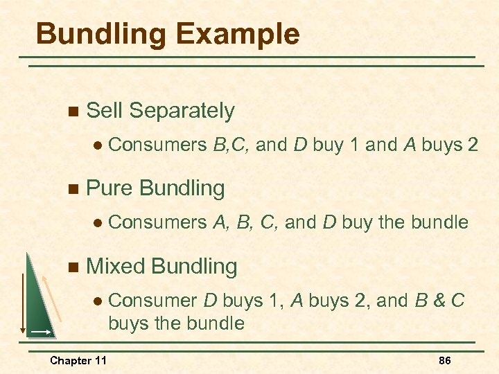Bundling Example n Sell Separately l n Pure Bundling l n Consumers B, C, and D buy 1 and A buys 2 Consumers A, B, C, and D buy the bundle Mixed Bundling l Chapter 11 Consumer D buys 1, A buys 2, and B & C buys the bundle 86

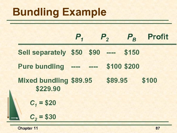Bundling Example P 1 P 2 Sell separately $50 $90 ---Pure bundling ---- Mixed bundling $89. 95 $229. 90 PB Profit $150 $100 $200 $89. 95 $100 C 1 = $20 C 2 = $30 Chapter 11 87

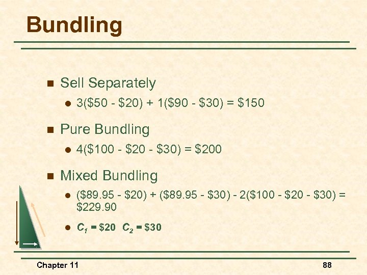Bundling n Sell Separately l n Pure Bundling l n 3($50 - $20) + 1($90 - $30) = $150 4($100 - $20 - $30) = $200 Mixed Bundling l ($89. 95 - $20) + ($89. 95 - $30) - 2($100 - $20 - $30) = $229. 90 l C 1 = $20 C 2 = $30 Chapter 11 88

Bundling n Question l If MC = 0, would mixed bundling still be the most profitable strategy with perfect negative correlation? Chapter 11 89

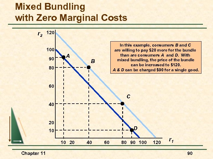Mixed Bundling with Zero Marginal Costs r 2 120 In this example, consumers B and C are willing to pay $20 more for the bundle than are consumers A and D. With mixed bundling, the price of the bundle can be increased to $120. A & D can be charged $90 for a single good. 100 90 A B 80 60 C 40 20 D 10 10 20 Chapter 11 40 60 80 90 100 120 r 1 90

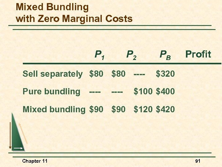Mixed Bundling with Zero Marginal Costs P 1 P 2 Sell separately $80 ---Pure bundling ---- PB Profit $320 $100 $400 Mixed bundling $90 $120 $420 Chapter 11 91

Bundling n Question l Why is mixed bundling more profitable with MC = 0? Chapter 11 92

Bundling n Bundling in Practice l Automobile option packages l Vacation travel l Cable television Chapter 11 93

Bundling n Mixed Bundling in Practice l Use of market surveys to determine reservation prices l Design a pricing strategy from the survey results Chapter 11 94

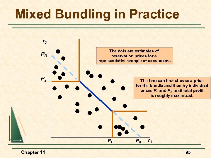Mixed Bundling in Practice r 2 PB The dots are estimates of reservation prices for a representative sample of consumers. P 2 The firm can first choose a price for the bundle and then try individual prices P 1 and P 2 until total profit is roughly maximized. P 1 Chapter 11 PB r 1 95

The Complete Dinner Versus a la Carte: A Restaurant’s Pricing Problem n Pricing to match consumer preferences for various selections n Mixed bundling allows the customer to get maximum utility from a given expenditure by allowing a greater number of choices. Chapter 11 96

Bundling n Tying l Practice of requiring a customer to purchase one good in order to purchase another. l Examples u u Chapter 11 Xerox machines and the paper IBM mainframe and computer cards 97

Bundling n Tying l Allows the seller to meter the customer and use a two-part tariff to discriminate against the heavy user l Mc. Donald’s u Chapter 11 Allows them to protect their brand name. 98

Advertising n Assumptions l Firm sets only one price l Firm knows Q(P, A) u Chapter 11 How quantity demanded depends on price and advertising 99

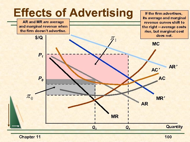Effects of Advertising AR and MR are average and marginal revenue when the firm doesn’t advertise. $/Q If the firm advertises, its average and marginal revenue curves shift to the right -- average costs rise, but marginal cost does not. MC P 1 AR’ AC’ P 0 AC MR’ AR MR Q 0 Chapter 11 Q 1 Quantity 100

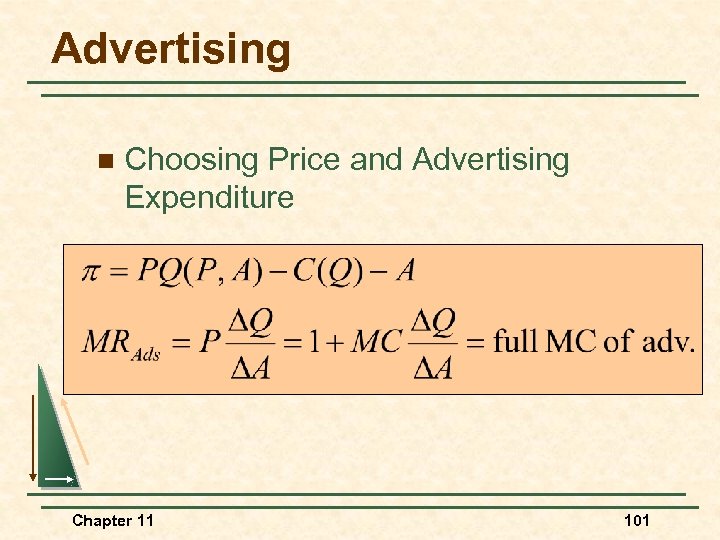Advertising n Choosing Price and Advertising Expenditure Chapter 11 101

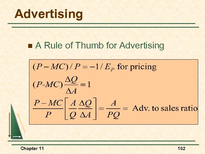Advertising n A Rule of Thumb for Advertising Chapter 11 102

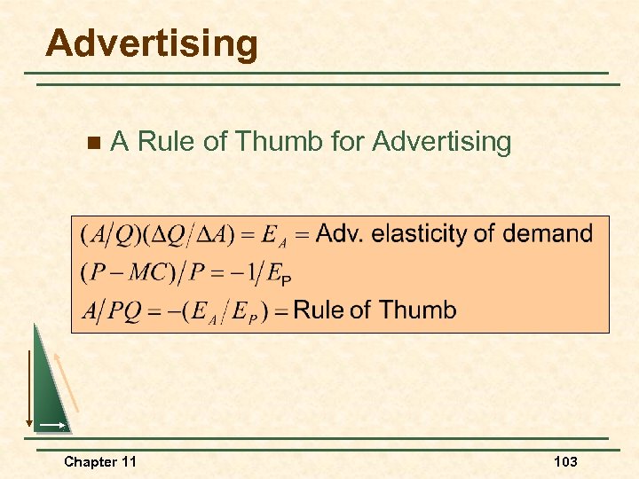Advertising n A Rule of Thumb for Advertising Chapter 11 103

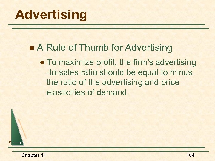Advertising n A Rule of Thumb for Advertising l Chapter 11 To maximize profit, the firm’s advertising -to-sales ratio should be equal to minus the ratio of the advertising and price elasticities of demand. 104

Advertising n An Example l R(Q) = $1 million/yr l $10, 000 budget for A (advertising--1% of revenues) l EA =. 2 (increase budget $20, 000, sales increase by 20% l EP = -4 (markup price over MC is substantial) Chapter 11 105

Advertising n Question l Should Chapter 11 the firm increase advertising? 106

Advertising n YES l A/PQ = -(2/-. 4) = 5% l Increase budget to $50, 000 Chapter 11 107

Advertising n Questions l When EA is large, do you advertise more or less? l When EP is large, do you advertise more or less? Chapter 11 108

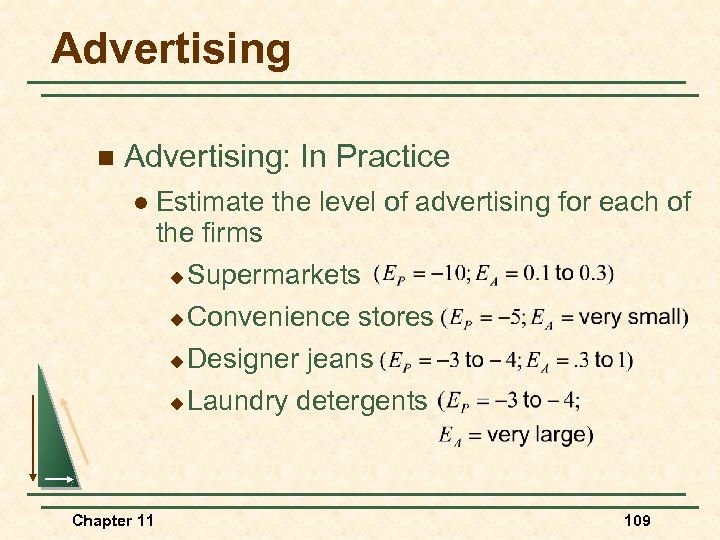Advertising n Advertising: In Practice l Chapter 11 Estimate the level of advertising for each of the firms u Supermarkets u Convenience stores u Designer jeans u Laundry detergents 109

Summary n Firms with market power are in an enviable position because they have the potential to earn large profits, but realizing that potential may depend critically on the firm’s pricing strategy. n A pricing strategy aims to enlarge the customer base that the firm can sell to, and capture as much consumer surplus as possible. Chapter 11 110

Summary n Ideally, the firm would like to perfectly price discriminate. n The two-part tariff is another means of capturing consumer surplus. n When demands are heterogeneous and negatively correlated, bundling can increase profits. Chapter 11 111

Summary n Bundling is a special case of tying, a requirement that products be bought or sold in some combination. n Advertising can further increase profits. Chapter 11 112

End of Chapter 11 Pricing with Market Power Chapter 11 113