Chapter 11 Oligopoly and Monopolistic Competition Table

Зарегистрируйтесь, чтобы просмотреть полный документ!

Chapter 11 Oligopoly and Monopolistic Competition

Table of Contents • • 11 -2 11. 1 11. 2 11. 3 11.

Introduction • Managerial Problem – Airbus and Boeing are the only two manufacturers of large commercial aircrafts. – If only one receives a government subsidy, how can it gain competitive advantage? What is the subsidy’s effect on p and q? What happens if both governments subsidize their firms? Should both firms lobby for government subsidies that result in a subsidy war? • Solution Approach – We need to focus on two markets. An oligopolistic market has few sellers and barriers to entry, firms have market power and may or may not collude to form cartels. A monopolistic competitive market has firms with market power, but there is free entry in the long run. • Empirical Methods – Within a cartel, oligopoly firms collude to raise prices and profits toward monopoly levels. – Oligopoly firms can independently set quantities (Cournot Model) or prices (Bertrand Model). – In monopolistic competitive markets, firms charge prices above marginal cost but make no economic profit in the long run. 11 -3 © 2014 Pearson Education, Inc. All rights reserved.

11. 1 Cartels • Cartel Objective: Higher Profits – Oligopolistic firms have an incentive to form cartels in which they collude in setting prices or quantities so as to increase their profits. – The Organization of Petroleum Exporting Countries (OPEC) is a wellknown example of an international cartel. • Cartel Basic Functioning – Typically, each member of a cartel agrees to reduce its output from the level it would produce if it acted independently. As a result, the market price rises and the firms earn higher profits. If the firms reduce market output to the monopoly level, they achieve the highest possible collective profit. – However, each member has an incentive to cheat. 11 -4 © 2014 Pearson Education, Inc. All rights reserved.

11. 1 Cartels • Why Cartels Form – A cartel forms if members of the cartel believe that they can raise their profits by coordinating their actions. – A cartel takes into account how changes in any one firm’s output affect the profits of all members of the cartel. Therefore, the aggregate profit of a cartel can exceed the combined profits of the same firms acting independently. • Competitive Market versus Cartel – In Figure 11. 1, there are n competitive firms and no further entry is possible. – In panel b, at the point of competitive equilibrium, the market output is Qc = nqc and price is pc. In panel a each firm takes pc and produces qc = Qc /n. – If the n firms form a cartel and act like a monopoly, the market output reduces to Qm but the price goes up to pm in panel b. The cartel profit increases and individual profits go up if firms charge pm and reduce output to qm in panel a. 11 -5 © 2014 Pearson Education, Inc. All rights reserved.

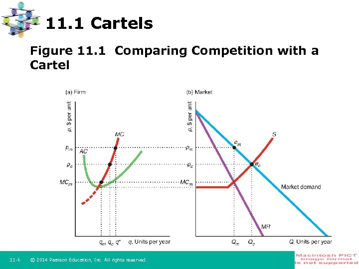
11. 1 Cartels Figure 11. 1 Comparing Competition with a Cartel 11 -6 ©

11. 1 Cartels • Why Cartels Fail: External Reasons – Cartels are generally illegal in developed countries. High fines and jail terms may prevent collusion. – Some cartels fail because they do not control enough of the market to significantly raise the price. • Why Cartels Fail: Internal Reasons – Cartel members have incentives to cheat if a member thinks its firm is just one of many firms so its extra output hardly affects the market price and the other firms in the cartel can’t tell who is producing more. – In panel a of Figure 11. 1, each firm agreed to qm. However, a price taker firm maximizes profit selling q*, where pm= MC. It makes extra money by producing more than qm, as long as MR > MC. – As more and more firms cheat, pm falls. Eventually, the cartel collapses. 11 -7 © 2014 Pearson Education, Inc. All rights reserved.

11. 1 Cartels • Maintaining Cartels: Cheating Detection – Some cartels may give members the right to inspect each other’s accounts or divide the market by region or by customers. – Cartels may turn to industry organizations to collect data on a firm’s market share. • Maintaining Cartels: Enforcement – Most-favored-customer clause: the seller would not offer a lower price to any other current or future buyer without offering the same price decrease to the firms that signed these contracts. • Maintaining Cartels: Government and Barriers to Entry – Sometimes governments help create and enforce cartels, exempting them from antitrust and competition laws. – The fewer the firms in a market, high barriers to entry, the more likely it is that other firms will know if a given firm cheats and the easier it is to impose penalties. 11 -8 © 2014 Pearson Education, Inc. All rights reserved.

11. 2 Cournot Oligopoly • Cournot Model – Assumptions: small number of firms and no entry, identical costs and identical products, firms set their quantities independently and simultaneously. – Because the firms set quantities, the price adjusts as needed until the market clears and profits are interdependent. • Residual Demand Best Responses – Firms use their residual demand curves: market demand that is not met by other sellers at any given price, Dr(p) = D(p) – So(p). – A firm maximizes profit with best responses that come from MRr = MC. • Equilibrium called Nash-Cournot Equilibrium – A set of quantities chosen by firms such that, holding the quantities of all other firms constant, no firm can obtain a higher profit by choosing a different quantity. – The quantity of equilibrium must be on the best response curve for all firms. 11 -9 © 2014 Pearson Education, Inc. All rights reserved.

11. 2 Cournot Oligopoly • Airlines: Residual Demand – The strategies for American and United depend on their residual demand curves and marginal costs. – If American thinks United flies q. U passengers, American’s residual demand is q. A = Q(p) – q. U. Alternatively, United’s residual demand is q. U = Q(p) – q. A • Airlines: Best Responses – To maximize profit, American sets MRr=MC and finds its best response curve for all possible q. U. Figure 11. 3 shows that if q. U = 64, American’s best response is q. A = 64, shuts down if q. U = 192, and so on. It also shows United’s best response curve. • Airlines: Nash-Cournot Equilibrium – There is only one pair of outputs where both firms are on their bestresponse curves, q. A = q. U = 64. At this intersection both firms maximize profits, are on their best response curves, and don’t want to change their outputs. 11 -10 © 2014 Pearson Education, Inc. All rights reserved.

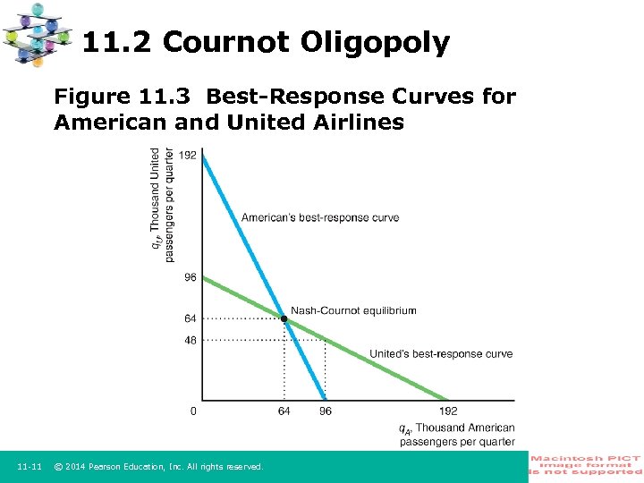
11. 2 Cournot Oligopoly Figure 11. 3 Best-Response Curves for American and United Airlines

11. 2 Cournot Oligopoly • Residual Demand, MR and MC – The market demand function is Q = 339 – p. The residual demand function for American is q. A = (339 – p) – q. U or p = 339 – q. A – q. U. – American’s marginal revenue function is MRr = 339 – 2 q. A – q. U. – Both airlines have MC = AC = $147 per passenger per flight. • MR = MC and Best Responses – MRr = MC, so 339 – 2 q. A – q. U = 147 – American’s best-response: q. A = 96 – 0. 5 q. U – Similarly, United’s best response: q. U = 96 – 0. 5 q. A • Nash-Cournot Equilibrium – Solving the two best responses by substitution, q. A = 96 – 0. 5 (96 – 0. 5 q. A ) – The Nash-Cournot equilibrium values: q. A = q. U = 64, Q= q. A + q. U = 128, p=$211 11 -12 © 2014 Pearson Education, Inc. All rights reserved.

11. 2 Cournot Oligopoly • Airlines with Calculus: Inverse Residual Demand, MR and MC – – The market demand function is Q = 339 – p The residual demand function for American is q. A = (339 – p) – q. U Inverse residual demand is p = 339 – q. A – q. U American’s revenue function: RA = pq. A = (339 – q. A – q. U)q. A= 339 q. A – q 2 A – q. U q. A – American’s marginal revenue function: MRr = d. RA/dq. A= 339 – 2 q. A – q. U – United’s revenue function: RU = 339 q. U – q 2 U – q. Uq. A – United’s marginal revenue function: MRr = d. RU/dq. U= 339 – 2 q. U – q. A • Best Responses and Nash-Cournot Equilibrium – Same steps and calculations as presented in the algebraic approach. 11 -13 © 2014 Pearson Education, Inc. All rights reserved.

11. 2 Cournot Oligopoly • The Number of Firms Matter – If two Cournot firms set output independently, the price to consumers is lower than the monopoly price. If there are more than two, the price is even lower. • Individual Output and Total Output – Consider the airlines’ inverse market demand function p = 339 – Q and n identical firms with MC=AC=$147. – The best response for any firm is q = 96 – [n – 1]q. So, q= 192/(n+1) – Total output is Q = qn = 192 n/(n+1) • Number of Firms and Nash-Cournot Equilibrium – If n = 1, Q = (192 × 1)/2 = 64, p = 243, a monopoly outcome. – If n = 2, Q = (192 × 2)/3 = 128, p = 211, a duopoly outcome as we found earlier. – If n is very large, Q = 192 and p = 147 = MC. The Nash-Cournot equilibrium approaches the competitive outcome. 11 -14 © 2014 Pearson Education, Inc. All rights reserved.

11. 2 Cournot Oligopoly • Non Identical Firms: Unequal Costs Case – In the Cournot model, a firm’s best-response function comes from MR = MC. If MC rises or falls, then the firm’s best-response function shifts. – Consider the Airline example, products are not differentiated, so American and United charge the same price. United’s MC drops from $147 to $99. • Best Responses – There is no change for American’s best-response. – United’s MRr curve is unaffected, but its best-response function shifts to the right in panel b of Figure 11. 4. United wants to produce more than before for any given level of American’s output. • Nash-Cournot Equilibrium – In panel b of Figure 11. 4, the Nash-Cournot equilibrium shifts from e 1 (both firms sold 64) to e 2, at which United sells 96 and American sells 48. – United’s profit increases from $4. 1 million to $9. 2 million, while American’s profit falls to $2. 3 million. Consumers also win because p falls from $211 to $195. 11 -15 © 2014 Pearson Education, Inc. All rights reserved.

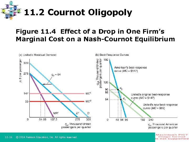
11. 2 Cournot Oligopoly Figure 11. 4 Effect of a Drop in One Firm’s

11. 2 Cournot Oligopoly • Non Identical Firms: Differentiated Products Case – By differentiating its product from those of a rival, an oligopolistic firm can shift its demand curve to the right and make it less elastic. – The less elastic the demand curve, the more the firm can charge because consumers are willing to pay more for a product that ‘seems’ superior. • Higher Prices and Choices – Although differentiation leads to higher prices, which harm consumers, differentiation is desirable in its own right. Consumers value having a choice, and some may greatly prefer a new brand to existing ones. • Nash-Cournot Equilibrium – If consumers think products differ, the Cournot quantities and prices may differ across firms. Each firm faces a different inverse demand function and hence charges a different price. 11 -17 © 2014 Pearson Education, Inc. All rights reserved.

11. 2 Cournot Oligopoly • Mergers – Mergers could be vertical or horizontal and both want to increase profit. – Vertical mergers may lower cost with a more efficient supply chain organization. Horizontal mergers may increase market power and reduce competition. • More Market Power May Not Be Enough – Cournot with 3 firms: Using Q=192 n/(n+1), each firm flies 48 k passengers, p=$195 and earns $2. 3 million. – Two firms merge, Cournot duopoly: Now, each of the remaining two firms flies 64 k passengers and earns $4. 1 million. Bad for the merged firms ($2. 05 < $2. 3). • Cost Advantage Pays Off – If the merger results in even a modest cost advantage, the merger may be worthwhile. In our example, if MC of the merged firms drops from $147 to $138, profit becomes $4. 9 million. Great for the merged firms ($2. 45 > $2. 3). – In general, the reduction in the number of firms may raise price insufficiently to make a merger profitable unless there is cost reduction. 11 -18 © 2014 Pearson Education, Inc. All rights reserved.

11. 3 Bertrand Oligopoly • Setting Prices - Oligopoly firms set prices and then consumers decide how many units to buy. The Bertrand equilibrium differs from the Cournot equilibrium; it depends on whether firms produce identical or differentiated products. • Best Responses – In a duopoly setting, Firm 1’s best response curve comes from answering “What is Firm 1’s best response—what price should it set—if Firm 2 sets a price of p 2 = x? ” for all possible values of x. – Similarly, Firm 2’s best response curve: “What is Firm 2’s best response (p 2) if Firm 1 sets a price of p 1 = y? ” for all possible values of y. • Nash-Bertrand Equilibrium – Nash-Bertrand equilibrium: a set of prices such that no firm can obtain a higher profit by choosing a different price if the other firms continue to charge these prices. 11 -19 © 2014 Pearson Education, Inc. All rights reserved.

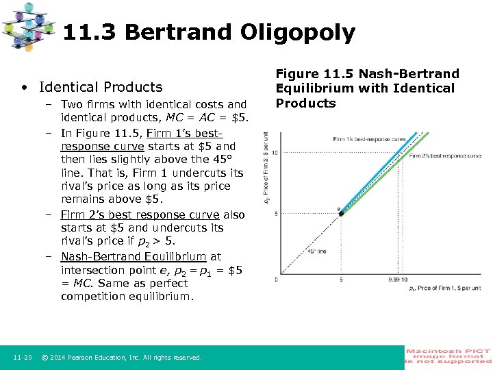
11. 3 Bertrand Oligopoly • Identical Products – Two firms with identical costs and identical products, MC = AC = $5. – In Figure 11. 5, Firm 1’s bestresponse curve starts at $5 and then lies slightly above the 45° line. That is, Firm 1 undercuts its rival’s price as long as its price remains above $5. – Firm 2’s best response curve also starts at $5 and undercuts its rival’s price if p 2 > 5. – Nash-Bertrand Equilibrium at intersection point e, p 2 = p 1 = $5 = MC. Same as perfect competition equilibrium. 11 -20 © 2014 Pearson Education, Inc. All rights reserved. Figure 11. 5 Nash-Bertrand Equilibrium with Identical Products

11. 3 Bertrand Oligopoly • Bertrand versus Cournot with Identical Products - The Nash-Bertrand equilibrium differs substantially from the Nash-Cournot equilibrium. Zero profits (p = MC) versus positive profits (p > MC). - The Cournot model seems more realistic than the Bertrand model in two ways. • Bertrand’s “Competitive” Equilibrium is Implausible – In a market with few firms, why would the firms compete so vigorously that they would make no profit? – Oligopolies typically charge a higher price than competitive firms. So, the Nash-Cournot equilibrium is more plausible. • Bertrand’s Equilibrium Price Depends on Cost Only – The Nash-Cournot equilibrium price is sensitive to demand conditions and the number of firms as well as on cost. So, it is better to study homogeneous goods markets. 11 -21 © 2014 Pearson Education, Inc. All rights reserved.

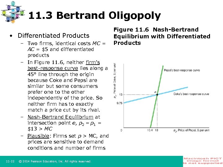
11. 3 Bertrand Oligopoly • Differentiated Products – Two firms, identical costs MC = AC = $5 and differentiated products – In Figure 11. 6, neither firm’s best-response curve lies along a 45° line through the origin because Coke and Pepsi are similar but some consumers prefer one to the other independently of the price. So neither firm has to exactly match a price cut by its rival. – Nash-Bertrand Equilibrium at intersection point e, p 2 = p 1 = $13 > MC – Plausible: Firms set p > MC, and prices are sensitive to demand conditions and number of firms 11 -22 © 2014 Pearson Education, Inc. All rights reserved. Figure 11. 6 Nash-Bertrand Equilibrium with Differentiated Products

11. 4 Monopolistic Competition • Monopoly/Oligopoly + Competitive Behavior - Monopolistic competition: market structure that has the price setting characteristics of monopoly or oligopoly and the free entry of perfect competition. These firms have oligopoly market power (face downward sloping demand curves), but earn zero profit due to free entry, as do perfectly competitive firms. • 1 st Reason for Downward Sloping Demand – Market demand may be limited so there is room for only few firms. So, the residual demand curve facing a single firm is downward sloping. – For example in a small town, the market may be large enough to support only a few plumbing firms, each of which provides a similar service. • 2 nd Reason for Downward Sloping Demand – Firms differentiate their products. So each firm can retain those customers who particularly like that firm’s product even if its price is higher than those of rivals. – For example, gourmet food trucks serve differentiated food in monopolistically competitive markets. 11 -23 © 2014 Pearson Education, Inc. All rights reserved.

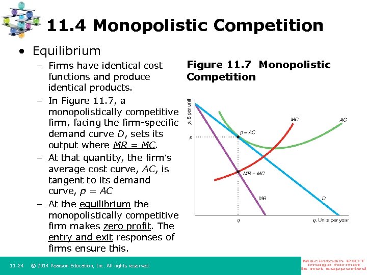
11. 4 Monopolistic Competition • Equilibrium Figure 11. 7 Monopolistic – Firms have identical cost functions and produce Competition identical products. – In Figure 11. 7, a monopolistically competitive firm, facing the firm-specific demand curve D, sets its output where MR = MC. – At that quantity, the firm’s average cost curve, AC, is tangent to its demand curve, p = AC – At the equilibrium the monopolistically competitive firm makes zero profit. The entry and exit responses of firms ensure this. 11 -24 © 2014 Pearson Education, Inc. All rights reserved.

11. 4 Monopolistic Competition • Profitability: If Identical Costs & Products, Zero Profit – If all firms in a monopolistically competitive market produce identical products and have identical costs: each firm earns zero economic profit in the long run. – Thus, all firms in the industry are on the margin of exiting the market because even a slight decline in profitability would generate losses. • Profitability: If Differentiated Costs & Products, Positive Profit – If those firms have different cost functions or produce differentiated products: most likely firms differ from each other in their profitability. – If so, low-cost firms or firms with superior products may earn positive economic profits in the long run. 11 -25 © 2014 Pearson Education, Inc. All rights reserved.

Managerial Solution • Managerial Problem – If only one receives a government subsidy, how can it gain competitive advantage? What is the subsidy’s effect on p and q? What happens if both governments subsidize their firms? Should both firms lobby for government subsidies that result in a subsidy war? • Solution – Assume Airbus and Boeing compete in a Cournot model, produce identical products with identical costs and face a linear demand curve. – A government per-unit subsidy to one firm would make its MC lower than its rival’s and its best-response curve shifts out. – If only Airbus is subsidized, Airbus should produce more given any expected output from Boeing. Airbus’ q and π rise while Boeing’s q and π fall. – If both governments give identical subsidies, both firms produce more, total Q increases, p falls (both move to competitive equilibrium) and both π fall. Each government is subsidizing final consumers in other countries without giving its own firm a competitive advantage. A subsidy war is not in these countries’ best interests. – However, these firms should not stop lobbying for subsidies to avoid being at a competitive disadvantage if its rival received a subsidy and it did not. 11 -26 © 2014 Pearson Education, Inc. All rights reserved.

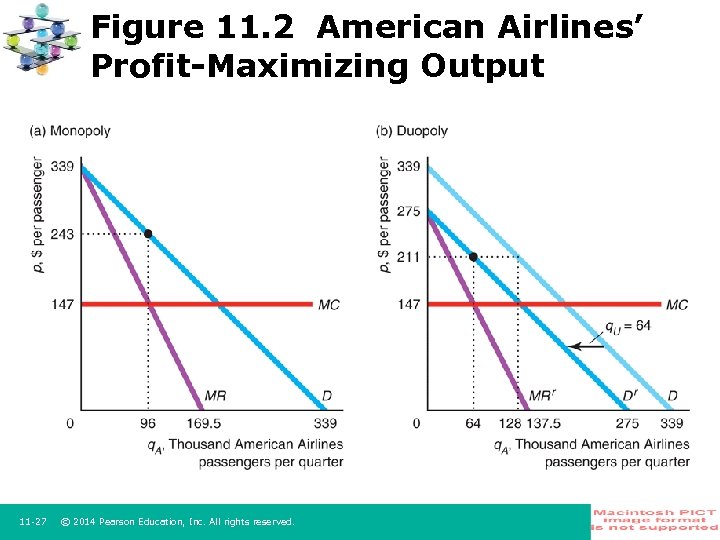
Figure 11. 2 American Airlines’ Profit-Maximizing Output 11 -27 © 2014 Pearson Education, Inc.

Скачать презентацию Chapter 11 Oligopoly and Monopolistic Competition Table

a4d0bd200ccec4f6c0a0be51128a38e5.ppt

Количество слайдов: 27