Chapter 11 Multiple Linear Regression Our Group

Chapter 11 Multiple Linear Regression

Our Group Members:

Content: ► Multiple Regression Model -----Yifan Wang ► Statistical Inference ---Shaonan Zhang & Yicheng Li ► Variable Selection Methods & SAS ---Guangtao Li & Ruixue Wang Strategy for Building a Model and Data Transformation --- Xiaoyu Zhang & Siyuan Luo ► Topics in Regression Modeling ----Yikang Chai & Tao Li ► ► Summary -----Xing Chen

Ch 11. 1 -11. 3 Introduction to Multiple Linear Regression Yifan Wang Dec. 6 th, 2007

Based on Chapter 10, we studied how to fit a linear relationship between a response variable y and a predictor variable x. But, sometimes we cannot handle a problem using simple linear regression, when there are two or more predictor variables. For Example The salary of a company employee may depend on l job category l years of experience l education l performance evaluations

Extend the simple linear regression model to the case of two or more predictor variables. Multiple Linear Regression (or simply Multiple Regression) is the statistical methodology used to fit such models.

Multiple Linear Regression In multiple regression we fit a model of the form (excluding the error term) Where are predictor variables and are k+1 unknown parameters. For example ear lin This model includes the kth degree polynomial model in a single variable x, namely, Since we can put .

11. 1 A Probabilistic Model For Multiple Linear Regression Regard the response variable as random Regard the predictor variables as nonrandom. The data for multiple regression consist of n vectors of observations ( ) for i =1, 2, …, n. Example 1 The response variable – the salary of the i th person in the sample The predictor variables – his/her years of experience – his/her years of education.

Example 2 is the observed value of the r. v. . predictor values depends on fixed according to the following model: Where is a random error with =0, and are unknown parameters. Assume are independent random variables. Then the are independent random variables with

11. 2 Fitting the Multiple Regression Model 11. 2. 1 Least Squares (LS) Fit The LS estimates of the unknown parameters minimize The LS can be found by setting the first partial derivatives of Q with respect to equal to zero. The result is a set of simultaneous linear equations in (k+1) unknowns. The resulting solutions, are the least squares (LS) estimates of , respectively estimates

11. 2. 2 Goodness of Fit of the Model To access the goodness of fit of the LS model, we use the residuals defined by Where the are the fitted values: An overall measure of the goodness of fit is the error sum of squares (SSE) Compare it to the total sum of squares (SST) As in Chapter 10, define the regression sum of squares (SSR) given by

the coefficient of multiple determination • , values closer to 1 represent better fits • Adding predictor variables generally increases , thus can be made to approach 1 by increasing the number of predictors. Multiple correlation coefficient (the positive square root coefficient of ): • only positive square root is used • r is a measure of the strength of the association between the predictor variables and the one response variable

11. 3 Multiple Regression Model in Matrix Notation The multiple regression model can be presented in a compact form by using matrix notation. Let be the n x 1 vectors of the r. v. ’s , their observed values , and random errors , respectively. Next let be the n x (k+1) matrix of the values of predictor variables.

Finally Let and be the (k + 1) x 1 vectors of unknown parameters and their LS estimates, respectively The model can be rewritten as: The simultaneous linear equations whose solutions yields the LS estimates can be written in matrix notation as If the inverse of the matrix exists, then the solution is given by

11. 4 Statistical Inference Shaonan Zhang & Yicheng Li

Statistical Inference on β’s ----General Hypothesis Test Determining the statistical significance of predictor variables we test the hypotheses: l if we can’t reject , can be dropped from the model

Statistical Inference on β’s ----General Hypothesis Test Pivotal Quantity recall: unbiased estimate of : l error degrees of freedom

Statistical Inference on β’s ----General Hypothesis Test Confidence Interval for Noted that l So, the CI is: where

Statistical Inference on β’s ----General Hypothesis Test P (Reject H 0 | H 0 is true) = Specially, when = 0, we reject H 0 if

Statistical Inference on β’s ----Another Hypothesis Test l Hypothesis: l Pivotal Quantity also, P-value If P-value is less than α, we reject H 0. And we use the previous test in this case. l

Statistical Inference on β’s ----Another Hypothesis Test l ANOVA Table for Multiple Regression Source of Variation (Source) Sum of Degrees of Mean F Squares Freedom Square (SS) (d. f. ) (MS) Regression SSR SSE SST Error Total k n - (k+1) n - 1

Statistical Inference on β’s ----Test Subsets of Parameters Full Model l Partial Model l l Hypothesis test statistics reject H 0 when

Prediction of Future Observations Let and l Whatever CI (Confidence Interval) or PI (Prediction Interval) we have and l Pivotal Quantity l l a (1 -) level CI to estimate *: l a (1 -) level PI to predict Y*:

11. 7 Variable Selection Methods Guangtao Li, Rui. Xue Wang

1. Why do we need variable selection methods? 2. Two methods are introduced v Stepwise Regression v Best Subsets Regression

11. 7. 1 STEPWISE REGRESSION Guangtao Li

Recall Test for Subsets of Parameters in 11. 4 • Full model: (i=1, 2, …n) • Partial model: (i=1, 2, …n) • Hypotheses: vs. for at least one • We test: • Reject H 0 when

► (p-1)-variable ► P-variable model:

Partial F-test: ► Reject H 0 p if

Partial Correlation Coefficients We should add to the regression equation only if is large enough, i. e. , only if is statistically significant.

Stepwise Regression Algorithm

SAS Program for the Algorithm ► Example: The Director of Broadcasting Operations for a television station wants to study the issue of “standby hours, ” which are hours where unionized graphic artists at the station are paid but are not actually involved in any activity. We are trying to predict the total number of Standby Hours per Week (Y). Possible explanatory variables are: Total Staff Present (X 1), Remote Hours(X 2), Dubner Hours (X 3) and Total Labor Hours (X 4). The results for 26 weeks are given below.

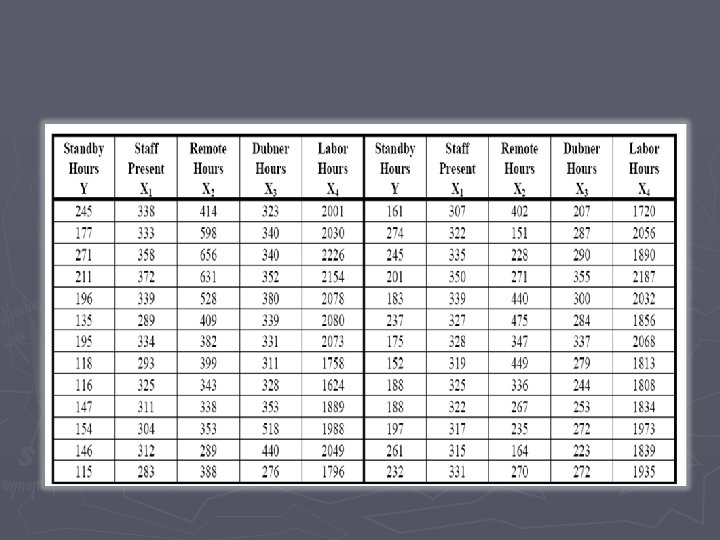
Data test; input y x 1 x 2 x 3 x 4; datalines; 245 338 414 177 333 598 271 358 656 211 372 631 196 339 528 135 289 409 195 334 382 118 293 399 116 325 343 147 311 338 154 304 353 146 312 289 115 283 388 323 340 352 380 339 331 311 328 353 518 440 276 2001 2030 2226 2154 2078 2080 2073 1758 1624 1889 1988 2049 1796

► ► ► ► ► 161 307 402 207 1720 274 322 151 287 2056 245 335 228 290 1890 201 350 271 355 2187 183 339 440 300 2032 237 327 475 284 1856 175 328 347 337 2068 152 319 449 279 1813 188 325 336 244 1808 188 322 267 253 1834 197 317 235 272 1973 261 315 164 223 1839 232 331 270 272 1935 run; proc reg data=test; model y = x 1 x 2 x 3 x 4 /SELECTION =stepwise ; run;

Selected SAS Output Stepwise Selection: Step 1 Variable x 1 Entered: R-Square = 0. 3660 and C(p) = 13. 3215 Analysis of Variance Sum of Mean Source DF Squares Square F Value Pr > F Model 1 20667 13. 86 0. 0011 Error 24 35797 1491. 55073 Corrected Total 25 56465 Parameter Standard Variable Estimate Error Type II SS F Value Pr > F Intercept -272. 38165 124. 24020 7169. 17926 4. 81 0. 0383 x 1 1. 42405 0. 38256 20667 13. 86 0. 0011 Bounds on condition number: 1, 1 -------------------------------------------

Stepwise Selection: Step 2 Variable x 2 Entered: R-Square = 0. 4899 and C(p) = 8. 4193 Analysis of Variance Sum of Mean Source DF Squares Square F Value Pr > F Model 27663 13831 11. 05 0. 0004 Error 23 28802 1252. 26402 Corrected Total 25 56465 Parameter Standard Variable Estimate Error Type II SS F Value Pr > F Intercept -330. 67483 116. 48022 10092 8. 06 0. 0093 x 1 1. 76486 0. 37904 27149 21. 68 0. 0001 x 2 -0. 13897 0. 05880 6995. 14489 5. 59 0. 0269

SAS Output(cont) ► All variables left in the model are significant at the 0. 1500 level. No other variable met the 0. 1500 significance level for entry into the model. Summary of Stepwise Selection ► ► Variable Step Entered 1 2 x 1 x 2 Variable Removed Number Partial Vars In R-Square 1 2 0. 3660 0. 1239 Model R-Square 0. 3660 0. 4899 C(p) 13. 3215 8. 4193 F Value 13. 86 5. 59 Pr > F 0. 0011 0. 0269

Ruixue Wang

11. 7. 2 Best Subsets Regression

11. 7. 2 Best Subsets Regression ►In practice there are often several almost equally good models, and the choice of the final model may depend on side considerations such as the number of variables, the ease of observing and/or controlling variables, etc. The best subsets regression algorithm permits determination of a specified number of best subsets of size p=1, 2, …, k from which the choice of the final model can be made by the investigator.

11. 7. 2 Best Subsets Regression Optimality Criteria Ø rp 2 -Criterion: Ø Adjusted rp 2 -Criterion: Ø Criterion: Some programs use minimization of as an optimization criterion. However, is not an independent criterion for it is equivalent to maximizing adjusted rp 2.

Ø Cp-Criterion (recommended for its ease of computation and its ability to judge the predictive power of a model) ►The sample estimator, Mallows’ Cpstatistic, is given by ► is an almost unbiased estimator of

PRESS p Criterion: The total prediction error sum of squares (press) is: This criterion evaluates the predictive ability of a postulated model by omitting one observation at a time, fitting the model based on the remaining observations and computing the predicted value for the omitted observation. The PRESS p criterion is intuitively easier to grasp than the Cp-Criterion , but it is computationally much more intensive and is not available in many packages.

SAS PRGRAM ► Data test; ► input y x 1 x 2 ► datalines; ► 245 338 ► 177 333 ► 271 358 ► 211 372 ► 196 339 ► 135 289 ► 195 334 ► 118 293 ► 116 325 ► 147 311 ► 154 304 ► 146 312 ► 115 283 x 4; 414 598 656 631 528 409 382 399 343 338 353 289 388 323 340 352 380 339 331 311 328 353 518 440 276 2001 2030 2226 2154 2078 2080 2073 1758 1624 1889 1988 2049 1796

SAS PRGRAM ► ► ► ► ► 161 307 402 207 1720 274 322 151 287 2056 245 335 228 290 1890 201 350 271 355 2187 183 339 440 300 2032 237 327 475 284 1856 175 328 347 337 2068 152 319 449 279 1813 188 325 336 244 1808 188 322 267 253 1834 197 317 235 272 1973 261 315 164 223 1839 232 331 270 272 1935 run; proc reg data=test; model y = x 1 x 2 x 3 x 4 /SELECTION =RSQUARE adjrsq CP mse ; run;

Results ► ► Number in Adjusted Model R-Square ► ► ► ► ► 1 0. 3660 0. 3396 13. 3215 1491. 55073 x 1 1 0. 1710 0. 1365 24. 1846 1950. 27491 x 4 1 0. 0597 0. 0205 30. 3884 2212. 24598 x 3 1 0. 0091 -. 0322 33. 2078 2331. 30545 x 2 -----------------------------------------2 0. 4899 0. 4456 8. 4193 1252. 26402 x 1 x 2 2 0. 4499 0. 4021 10. 6486 1350. 49234 x 1 x 3 2 0. 4288 0. 3791 11. 8231 1402. 24672 x 3 x 4 2 0. 3754 0. 3211 14. 7982 1533. 34044 x 1 x 4 2 0. 2238 0. 1563 23. 2481 1905. 67595 x 2 x 4 2 0. 0612 -. 0205 32. 3067 2304. 83375 x 2 x 3 -----------------------------------------3 0. 5378 0. 4748 7. 7517 1186. 29444 x 1 x 3 x 4 3 0. 5362 0. 4729 7. 8418 1190. 44739 x 1 x 2 x 3 3 0. 5092 0. 4423 9. 3449 1259. 69053 x 1 x 2 x 4 3 0. 4591 0. 3853 12. 1381 1388. 36444 x 2 x 3 x 4 -----------------------------------------4 0. 6231 0. 5513 5. 0000 1013. 46770 x 1 x 2 x 3 x 4 C(p) MSE Variables in Model

11. 7. 2 Best Subsets Regression & SAS The resource of the example is http: //www. math. udel. edu/teaching/course_materials/m 202_climent/Multiple%20 Regression%20%20 Model%20 Building. pdf

11. 5, 11. 8 Building A Multiple Regression Model by Si. Yuan Luo & Xiaoyu Zhang

Introduction • Building a multiple regression model consists of 7 steps. • Though it is not necessary to follow each and every step in exact sequence shown on the next slide, the general approach and major steps should be followed. • The model is an iterative process, it may take several cycles of the steps before arriving at the final model.

The “ 7 steps” 1. Decide the type 5. Fit candidate models 6. Select and evaluate 2. Collect the data 3. Explore the data 4. Divide the data 7. Select the final model

Step 1 Decide the type of model needed, different types of models includes: § Predictive – a model used to predict the response variable from a chosen set of predictor variables. § Theoretical – a model based on a theoretical relationship between a response variable and predictor variables. § Control – a model used to control a response variable by manipulating predictor variables. § Inferential – a model used to explore the strength of relationships between a response variable and individual predictor variables. § Data summary – a model used primarily as a device to summarize a large set of data by a single equation. ► Often a model can be used for multiple purposes. ► The type of model dictates the type of data needed. ►

Step 2 Collect the data ► Decide the variables (predictor and response) on which to collect data. Measurement of the variables should be done the right way depending on the type of subject. ► See chapter 3 for precautions necessary to obtain relevant, bias-free data.

Step 3 Explore the data ► The data should be examined for outliers, gross errors, missing values, etc. on a univariate basis using the techniques discussed in chapter 4. Outliers cannot just be omitted because much useful information can be lost. See chapter 10 for how to deal with outliers. ► Scatter plots should be made to study bivariate relationships between the response variable and each of the predictors. They are useful in suggesting possible transformations to linearize the relationships.

Step 4 Divide the data ► Divide the data into training and test sets: only a subset of the data, the training set, should be used to fit the model (step 5 and 6); the remainder, called the training set, should be used for cross-validation of the fitted model (step 7). ► The reason for using an independent data set to test the model is that if the same data are used for both fitting and testing, then an overoptimistic estimate of the predictive ability of the fitted model is obtained. ► The split for the two sets should be done randomly.

Step 5 fit Candidate models ► Generally several equally good models can be identified using the training data set. ► By conducts several runs by varying FIN and FOUT values, we can identify several that fits the training set.

Step 6 Select and evaluate ► From the list of candidate models we are now ready to select two or three good models based on criteria such as the Cp-statistic, the number of predictors (p), and the nature of predictors. ► These selected models should be checked for violation of model assumptions using standard diagnostic techniques, in particular, residual plots. Transformations in the response variable or some of the predictor variables may be necessary to improve model fits.

Step 7 Select the Final model: ► This is the step where we compare competing models by cross-validating them against the test data. ► The model with a smaller cross-validation SSE is better predictive model. ► The final selection of the model is based on a number of considerations, both statistical and no statistical. These include residual plots, outliers, parsimony, relevance, and ease of measurement of predictors. A final test of any model is that it makes practical sense and the client is willing to buy it.

Regression Diagnostics (Step VI) ► Graphical Analysis of Residuals § Plot Estimated Errors vs. Xi Values Between Actual Yi & Predicted Yi ►Estimated Errors Are Called Residuals ►Difference § Plot Histogram or Stem-&-Leaf of Residuals ► Purposes § Examine Functional Form (Linearity ) § Evaluate Violations of Assumptions

Linear Regression Assumptions ► Mean of Probability Distribution of Error Is 0 ► Probability Distribution of Error Has Constant Variance ► Probability Distribution of Error is Normal ► Errors Are Independent

Residual Plot for Functional Form (Linearity) Add X^2 Term Correct Specification

Residual Plot for Equal Variance Unequal Variance Correct Specification Fan-shaped. Standardized residuals used typically (residual divided by standard error of prediction)

Residual Plot for Independence Not Independent Correct Specification

Data transformations ► Why do we need data transformations? § Make seemingly nonlinear models linear example: § Sometimes it gives a better explanation of the variation in the data

► How do we do the data transformations? § Power family of transformations on the response : Box-Cox method ►Requirements: all the data is always positive The ratio of the largest observed Y to the smallest is at least 10

§ Transformation form V= where is the geometric mean of the

§ How to estimate ► 1. Choose a value of from a selected range. Usually we look for it in the range (-1, 1), we would usually cover the selected range with about 11 -21 values of ► 2. For each value, evaluate V by applying each Y to the formula above. You will create a vector V=( ), then use it to fit a linear model by least squares method. Record the residual sum of squares for the regression ► 3. Plot versus. Draw a smooth curve through the plotted points, and find at what value of the lowest point of the curve lies. That , is the maximum likelihood estimate of

► Example: § The data in table are part of a more extensive set given by Derringer(1974). This paper has been adapted with permission of John Wiley & Sons, Inc. we wish to find a transformation of the form , or , which will provide a good first-order fit to the data. Our model form is where f is the filler level and p is the plasticizer level.

Napht henic Oil, ph r, p 0 10 20 30 0 Filler, phr, f 12 24 36 48 60 26 17 13 ---- 38 26 20 15 108 83 57 41 157 124 87 63 50 37 27 22 76 53 37 27

§ Note that the response data range from 157 to 13, a ratio of 157/13=12. 1>10, hence a transformation on Y is likely to be effective. The geometric mean is 41. 5461 for this set of data. The next table shows a selected values of We pick 20 different values of from (-1, 1) in this case.

-1. 0 -0. 8 -0. 6 -0. 4 -0. 2 -0. 15 -0. 10 -0. 08 -0. 06 -0. 05 2456 1453 779. 1 354. 7 131. 7 104. 5 88. 3 84. 9 83. 3 83. 2 -0. 04 -0. 02 0. 00 0. 05 0. 10 0. 2 0. 4 0. 6 0. 8 1. 0 83. 5 85. 5 89. 3 106. 7 135. 9 231. 1 588. 0 1222 2243 3821

§ A smooth curve through these points is plotted in the next figure. We see that the minimum occurs at about =0. 05. This is close to zero, so suggesting that the transformation V= , or more simply.

§ Application of the transformation to the original data, then we get a set of data which are better linearly related. The best plane, fitted to these transformed data by least squares, is =3. 212+0. 03088 f-0. 03152 p. the ANOVA table for this model is Source , | Residual Total Df SS 1 2 20 23 319. 44855 ----- 10. 51667 5. 27583 0. 05171 0. 00258 330. 05193 MS F 2045

§ If we had fitted a first-order model to the untransformed data, we will obtain =28. 184+1. 55 f-1. 717 p ANOVA table for this model Source , | Residual Total, corrected Df 2 20 22 SS MS F 27842. 62 13921. 31 72. 9 3820. 60 191. 03 31663. 22

► We find out the transformed model has much stronger Fvalue.

11. 6. 1 -11. 6. 3 Topics in Regression Modeling Yikang Chai & Tao Li

11. 6. 1 Multicollinearity Def. The columns of the X matrix are exactly or approximately linearly dependent. It means the predictor variables are related. ► why are we concerned about it? This can cause serious numerical and statistical difficulties in fitting the regression model unless “extra” predictor variables are deleted. ►

How does the multicollinearity cause difficulties? The multicollinearity leads to the following problems: 1. is nearly singular, which makes numerically unstable. This reflected in large changes in their magnitudes with small changes in data. 2. The matrix has very large elements. Therefore are large, which makes statistically nonsignificant.

Measures of Multicollinearity Three ways: 1. The correlation matrix R. Easy but can’t reflect linear relationships between more than two variables. 2. Determinant of R can be used as measurement of singularity of. 3. Variance Inflation Factors (VIF): the diagonal elements of . Generally, VIF>10 is regarded as unacceptable.

11. 6. 2 Polynomial Regression Consider the special case: Problems: 1. The powers of x, i. e. , tend to be highly correlated. 2. If k is large, the magnitudes of these powers tend to vary over a rather wide range. These problems lead to numerical errors.

How to solve these problems? Two ways: 1. Centering the x-variable: Removing the non-essential multicollinearity in the data. 2. Standardize the x-variable: Alleviate the problem that x varying over a wide range.

11. 6. 3 Dummy Predictor Variables It’s an method to deal with the categorical variables. 1. For ordinal categorical variables, such as the prognosis of a patient (poor, average, good), just assign numerical scores to the categories. (poor=1, average=2, good=3) 2. If we have nominal variable with c>=2 categories. Use c-1 indicator variables, , called Dummy Variables, to code.

How to code? set for the ith category, for the cth category. Why don’t we just use c indicator variables: ? because there will be a linear dependency among them: This will cause multicollinearity.

Example The season of a year can be coded with three indicators: x 1(winter), x 2(spring), x 3(summer). With this coding (1, 0, 0)for Winter , (0, 1, 0) for Spring, (0, 0, 1) for Summer and (0, 0, 0) for Fall Consider modeling the temperature of a year of an area as a function of the season (X) and its latitude (A) , we can get the following model: For winter: For summer: For spring: For fall:

Logistic Regression Model 1938, By R. A. Fisher and Frank Yates ► Logistic transform for analyzing binary data. ►

Logistic Regression Model ► The Importance of Logistic Regression Model 1. Logistic regression model is the most popular model for binary data. 2. Logistic regression model is generally used for binary response variables. Y = 1 (true, success, YES, etc. ) , while Y = 0 ( false, failure, NO, etc. )

Logistic Regression Model Details of Regression Model Main Step 1. Consider a response variable Y {0 or 1} and a single predictor variable x. 2. Model E(Y|x) =P(Y=1|x) as a function of x. The logistic regression model expresses the logistic transform of P(Y=1|x). ►

Logistic Regression Model ► Example i X 28 29 30 31 32 33 Ii iii Instances of Y Coded as 0 4 3 2 2 4 1 2 2 7 7 16 14 iv Total ii+iii 6 5 9 9 20 15 v vi vii Y as Log Observed Odds Probability Ratio. 3333. 5000 -. 6931 . 4000. 6667 -. 4055 . 7778 3. 5000 1. 2528 . 8000 4. 0000 1. 3863 . 9333 14. 0000 2. 6391 http: //faculty. vassar. edu/lowry/logreg 1. html

Logistic Regression Model A. Ordinary Linear Regression B. Logistic Regression

Logistic Regression Model ► Weighted Linear Regression of Observed Log Odds Ratios on X X 28 29 30 31 32 33 Observed 0. 3333 0. 4 0. 7778 0. 9333 Log -. 6931 -. 4055 1. 2528 1. 3863 2. 6391 Weight 6 5 9 9 20 15

Logistic Regression Model ► Properties of Regression Model E(Y|x) = P(Y=1| x) *1 + P(Y=0|x) * 0 = P(Y=1|x) is bounded between 0 and 1 for all values of x. While, it is not true if we use model: § In ordinary regression, the regression coefficient has the interpretation that it is the log of the odds ratio of a success event (Y=1) for a unit change in x. § ► Extension to Multiple predictor variables

Standardized Regression Coefficients ► Why we need standardize regression coefficients? Recall the regression equation for linear regression model: 1. 2. The magnitudes of the can not be directly used to judge the relative effects of on y. By using standardized regression coefficients, we may be able to judge the importance of different predictors

Standardized Regression Coefficients ► Standardized Transform ► Standardized Regression Coefficients

Standardized Regression Coefficients ► Example(Industrial sales data from text book) Linear Model: ► The regression equation: ► ► Notice: but thus has a much larger effect than on y

Chapter Summary Multiple linear regression model ► Fitting the multiple regression model Least squares fit ► Goodness of fit of the model – SSE, SST, SSR, r^2 Statistical inference for multiple regression 1. T-test ► 2. F-test for all for at least one 3. F-test for at least one How do we select variables (SAS)? Stepwise regression - it’s fancy algorithm ► Best subsets regression – more realistic, flexible How about if the data is not linear? Data transformation ► Building a multiple regression model – 7 steps ►

We very appreciate your attention =) Please feel free to ask questions.

The End Thank You!