Chapter 11 Input Markets and the Allocation of

Chapter 11 Input Markets and the Allocation of Resources 11/1 © 2009 Pearson Education Canada

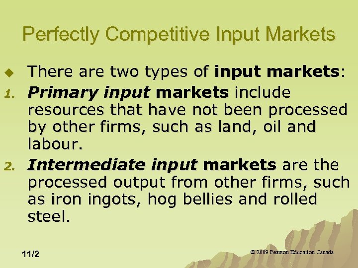Perfectly Competitive Input Markets u 1. 2. There are two types of input markets: Primary input markets include resources that have not been processed by other firms, such as land, oil and labour. Intermediate input markets are the processed output from other firms, such as iron ingots, hog bellies and rolled steel. 11/2 © 2009 Pearson Education Canada

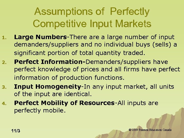Assumptions of Perfectly Competitive Input Markets 1. 2. 3. 4. Large Numbers-There a large number of input demanders/suppliers and no individual buys (sells) a significant portion of total quantity traded. Perfect Information-Demanders/suppliers have perfect knowledge of prices and all firms have perfect information of production functions. Input Homogeneity-In any input market, all units of the input are identical. Perfect Mobility of Resources-All inputs are perfectly mobile. 11/3 © 2009 Pearson Education Canada

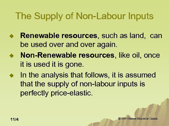The Supply of Non-Labour Inputs u u u 11/4 Renewable resources, such as land, can be used over and over again. Non-Renewable resources, like oil, once it is used it is gone. In the analysis that follows, it is assumed that the supply of non-labour inputs is perfectly price-elastic. © 2009 Pearson Education Canada

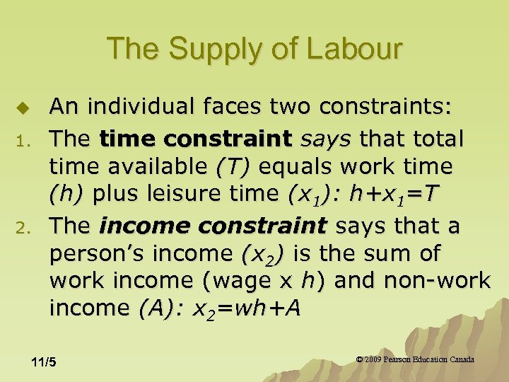The Supply of Labour u 1. 2. An individual faces two constraints: The time constraint says that total time available (T) equals work time (h) plus leisure time (x 1): h+x 1=T The income constraint says that a person’s income (x 2) is the sum of work income (wage x h) and non-work income (A): x 2=wh+A 11/5 © 2009 Pearson Education Canada

The Leisure-Income Constraint u The leisure income constraint: wx 1+x 2=A+w. T u The wage (w) is the price of leisure and the slope of the budget constraint. u A+w. T is full (all work) income. u The utility maximizing bundle of leisure/labour is where the indifference curve is tangent to the leisure-income constraint in Figure 11. 1 11/6 © 2009 Pearson Education Canada

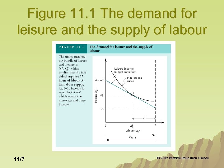Figure 11. 1 The demand for leisure and the supply of labour 11/7 © 2009 Pearson Education Canada

Figure 11. 2 Leisure as a normal good 11/8 © 2009 Pearson Education Canada

Figure 11. 3 Income and substitution effects for a wage change 11/9 © 2009 Pearson Education Canada

Response to a Change in Wage Rate When leisure is a normal good, the hours of work may increase or decrease in response to a wage increase, depending upon whether the income effect is greater than or less than the income effect. u When leisure is an inferior good, an increase in wage rate invariably leads to a decrease in leisure hours and an increase in work hours. u 11/10 © 2009 Pearson Education Canada

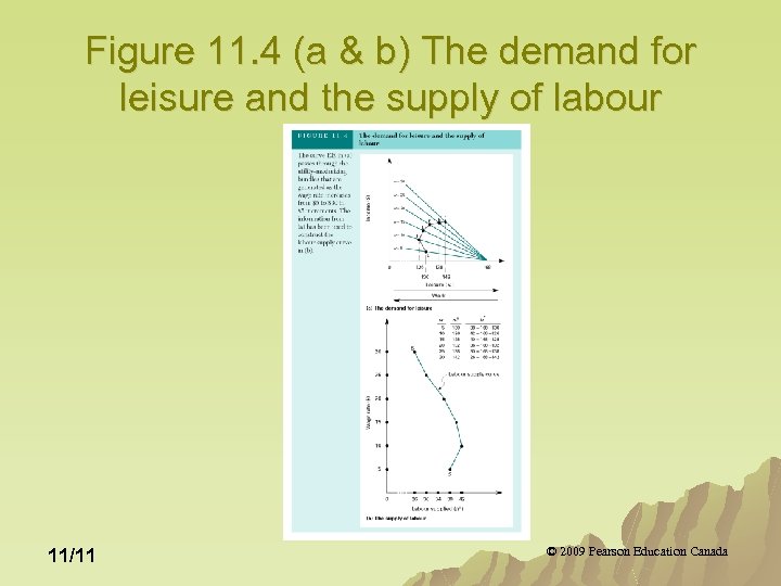Figure 11. 4 (a & b) The demand for leisure and the supply of labour 11/11 © 2009 Pearson Education Canada

Firm’s Demand for One Variable Input u The short-run demand function relates to a scenario where only one input is variable. 11/12 © 2009 Pearson Education Canada

Input Demand in a One-Good Economy u For any wage less than the maximum value of the average product, the firm’s demand function is the downward sloping portion of the marginal product curve. u For any wage rate greater than the maximum value of the average product, the firm maximizes profits by hiring no labour. 11/13 © 2009 Pearson Education Canada

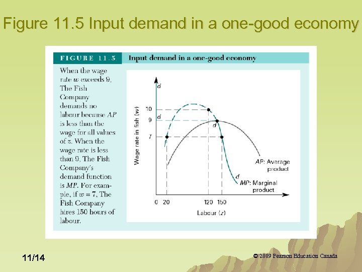Figure 11. 5 Input demand in a one-good economy 11/14 © 2009 Pearson Education Canada

Transforming the Product Curves into Revenue Curves u Marginal Revenue Product is the marginal product from an additional unit of labour times the marginal revenue when the additional output is sold: MRP(z)=MR(y)MP(z) u Similarly, Average Revenue Product equals the price of the output times average product of the variable input: ARP(z)=p. AP(z) 11/15 © 2009 Pearson Education Canada

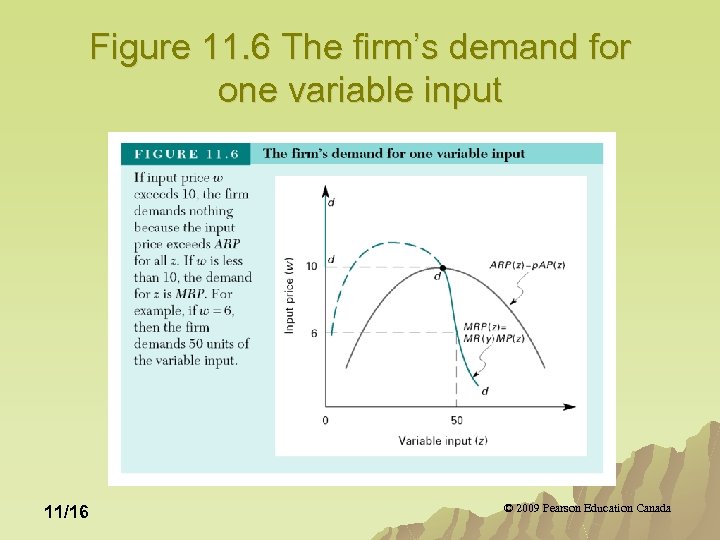Figure 11. 6 The firm’s demand for one variable input 11/16 © 2009 Pearson Education Canada

The Firm’s Demand Curve for One Variable Input For input prices less than the maximum values of ARP, the firm’s demand function is the downward-sloping portion of MRP. u For input prices greater than the maximum value of ARP, the firm will demand none of the variable input. u Given an initial positive quantity of the input demanded, an increase in the price of an input, will cause the firm to reduce the quantity demanded of that input. u 11/17 © 2009 Pearson Education Canada

The Firm’s Demand Curve for One Variable Input u The value of the marginal product (VMP) of the variable input (VMPz) is output price time marginal product: VMPz=p. MP(z). u For a perfect competitor, VMP =MRP (since p=MR). u For a monopoly, MRP

Input Demand with Many Variable Inputs u In the long run all inputs are variable. u In the long run, the firm’s response to an input price change will, via both the substitution effect and the output effect, produce a downward sloping input demand curve. 11/19 © 2009 Pearson Education Canada

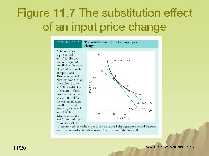Figure 11. 7 The substitution effect of an input price change 11/20 © 2009 Pearson Education Canada

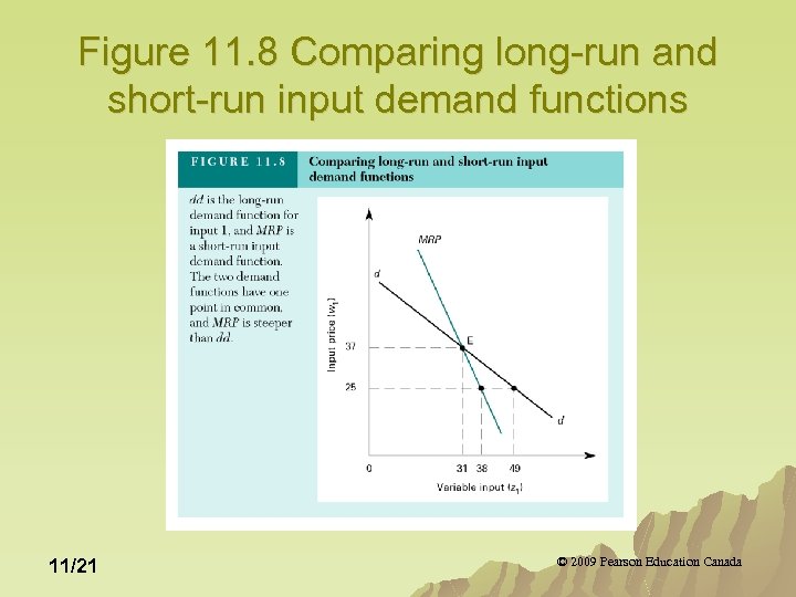Figure 11. 8 Comparing long-run and short-run input demand functions 11/21 © 2009 Pearson Education Canada

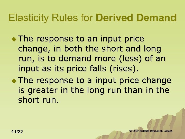Elasticity Rules for Derived Demand u The response to an input price change, in both the short and long run, is to demand more (less) of an input as its price falls (rises). u The response to a input price change is greater in the long run than in the short run. 11/22 © 2009 Pearson Education Canada

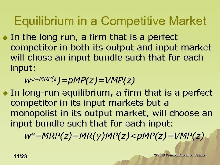Equilibrium in a Competitive Market In the long run, a firm that is a perfect competitor in both its output and input market will chose an input bundle such that for each input: we=MRP(z)=p. MP(z)=VMP(z) u In long-run equilibrium, a firm that is a perfect competitor in its input markets but a monopolist in its output market, will choose an input bundle such that for each input: we=MRP(z)=MR(y)MP(z)

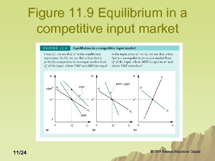Figure 11. 9 Equilibrium in a competitive input market 11/24 © 2009 Pearson Education Canada

Monopsony in Input Markets u. A monopsonist has significant control over what it pays for an input. u The relationship between input price (w) and quantity of the input (z) is determined by the market supply function for the input: w=S(w). 11/25 © 2009 Pearson Education Canada

Monopsony in Input Markets u The monopsonist buys all units of an input at the same price (average factor cost or AFC). u Total factor cost (TFC) is quantity (z) times AFC or price S(z): TFC(z)=z. S(z) 11/26 © 2009 Pearson Education Canada

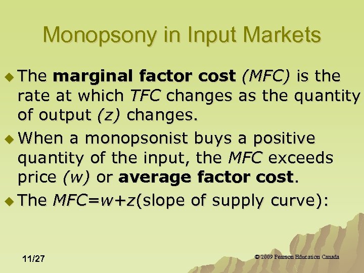Monopsony in Input Markets u The marginal factor cost (MFC) is the rate at which TFC changes as the quantity of output (z) changes. u When a monopsonist buys a positive quantity of the input, the MFC exceeds price (w) or average factor cost. u The MFC=w+z(slope of supply curve): 11/27 © 2009 Pearson Education Canada

Figure 11. 11 A monopsonist’s profit-maximizing decision 11/28 © 2009 Pearson Education Canada

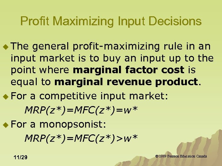Profit Maximizing Input Decisions u The general profit-maximizing rule in an input market is to buy an input up to the point where marginal factor cost is equal to marginal revenue product. u For a competitive input market: MRP(z*)=MFC(z*)=w* u For a monopsonist: MRP(z*)=MFC(z*)>w* 11/29 © 2009 Pearson Education Canada

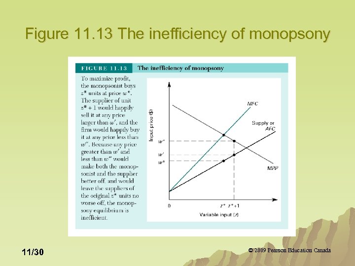Figure 11. 13 The inefficiency of monopsony 11/30 © 2009 Pearson Education Canada

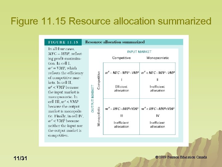Figure 11. 15 Resource allocation summarized 11/31 © 2009 Pearson Education Canada

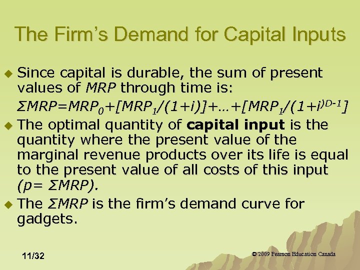The Firm’s Demand for Capital Inputs Since capital is durable, the sum of present values of MRP through time is: ΣMRP=MRP 0+[MRP 1/(1+i)]+…+[MRP 1/(1+i)D-1] u The optimal quantity of capital input is the quantity where the present value of the marginal revenue products over its life is equal to the present value of all costs of this input (p= ΣMRP). u The ΣMRP is the firm’s demand curve for gadgets. u 11/32 © 2009 Pearson Education Canada

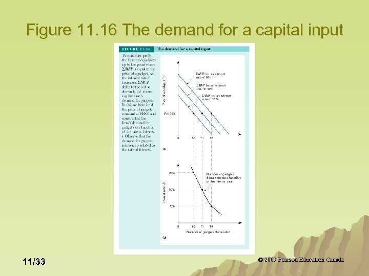Figure 11. 16 The demand for a capital input 11/33 © 2009 Pearson Education Canada

Human Capital Decisions Over Time u Human capital - investments in education and training. u Human capital production function: R=F(H) Which says additional income (return on human capital investment) (R), is a diminishing function of the quantity of human capital (H). 11/34 © 2009 Pearson Education Canada

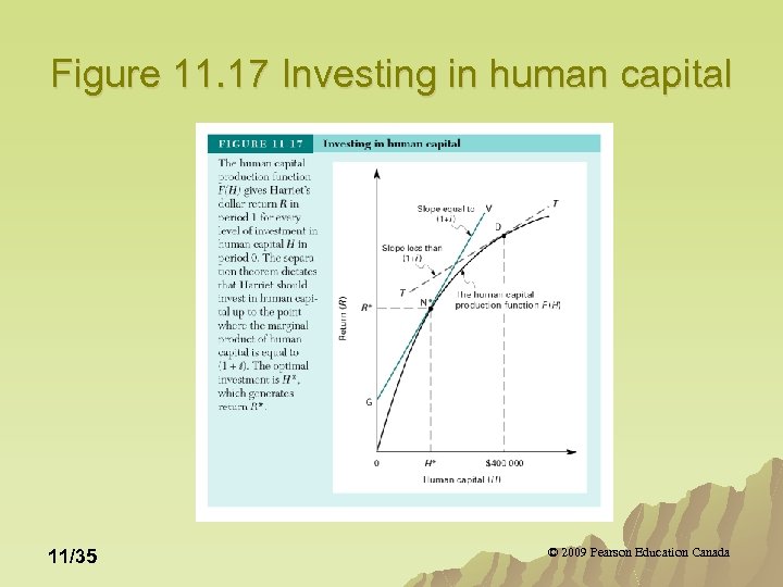Figure 11. 17 Investing in human capital 11/35 © 2009 Pearson Education Canada

From Figure 11. 17 u Invest in an additional dollar of human capital if the marginal product (MP) exceeds the rate at which current foregone consumption can generate future consumption (1+i). u To maximize the present value of net income, invest in human capital up to the point where MP=(1+i). 11/36 © 2009 Pearson Education Canada

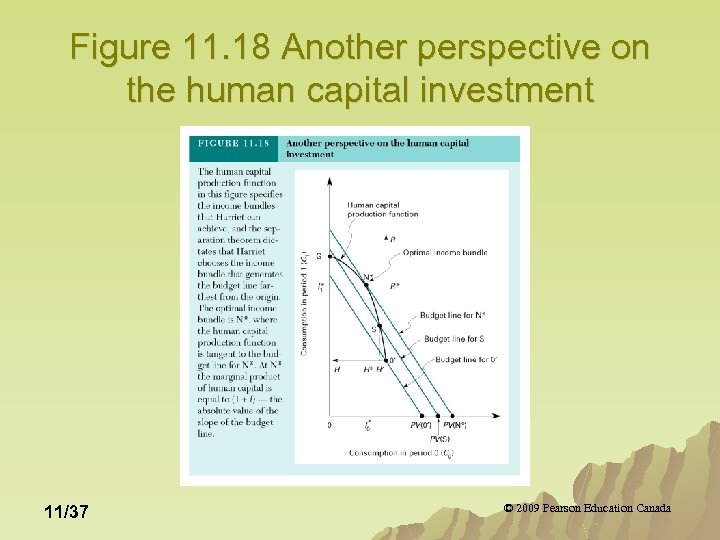Figure 11. 18 Another perspective on the human capital investment 11/37 © 2009 Pearson Education Canada

Figure 11. 19 The life-cycle choice 11/38 © 2009 Pearson Education Canada