Chapter 11 Forecasting Models 2007 Pearson Education

Chapter 11: Forecasting Models © 2007 Pearson Education

Forecasting • Forecasting is attempting to predict the future • Decision makers want to reduce uncertainty by predicting future values such as sales or investment return

Steps in Forecasting 1. 2. 3. 4. 5. 6. 7. Determine the objective of the forecast Identify items to be forecast Determine time horizon Select the forecasting model(s) Gather data Validate model Make forecast and implement results

Types of Forecasts 1. Qualitative - subjective methods based on intuition and experience 2. Time Series – based on historical data and assume the past indicates the future 3. Causal Models – data based where there may be a cause and effect relation between variables

Qualitative Forecasting Models 1. Delphi Method – an iterative group process where a group of experts attempt to reach consensus 2. Jury of Executive Opinion – uses opinions of high level managers often combined with statistical models

Qualitative Forecasting Models 3. Sales Force Composite – each salesperson estimates sale in his/her own region and forecast are combined for an overall forecast 4. Consumer Market Survey – future purchase plans are solicited from customers

Measuring Forecast Error Measures how accurate the forecast was For time period t: Forecast error = Actual value – Forecast value = A t - Ft

Methods of Measuring Overall Forecast Error • Mean Absolute Deviation (MAD) MAD = ∑ |At – Ft| / T where T = the number of time periods • Mean Squared Error (MSE) MSE = ∑ (At – Ft)2 / T

Methods of Measuring Overall Forecast Error • Mean Absolute Percent Error (MAPE) Measure error as a percent of actual values MAPE = 100 ∑ [ |At – Ft| / At ] / T

Time Series • • A time series is where the same value is recorded at regular time intervals Examples: daily stock price, monthly sales, annual revenue, etc.

Components of a Time Series 1. Trend – long term upward or downward movement 2. Seasonality – the pattern that occurs every year 3. Cycles – the pattern that occurs over a period of years 4. Random variations – caused by chance and unusual events

Time Series Components

Time Series Decomposition • • A time series can be broken down into its individual components Two approaches: 1. Multiplicative decomposition Forecast = Trend x Seasonality x Cycles x Random 2. Additive decomposition Forecast = Trend + Seasonality + Cycles + Random

Stationary and Nonstationary Time Series Data • If a time series has an upward or downward trend, it is nonstationary • If it has no trend, it is stationary

Moving Averages • Smooth out variations in a time series when values are fairly steady • Some number (k) of consecutive periods are averaged k-period moving average = ∑ (actual values in previous k periods) k

Wallace Garden Supply Example

Weighted Moving Averages A moving average where some periods are weighted more heavily than others K-period weighted moving average = ∑ (wi Ai) / ∑ (wi) where, wi = weight for period i Ai = actual value for period i

Wallace Garden Supply With Weighted Moving Averages Period last month 2 month ago 3 months ago Weights 3 2 1

3 -Month Weighted Moving Average

Using Solver to Find the Optimal Weights • The weights are the decision variables (changing cells) • Minimize some measure of forecast error (MAD, MSE, or MAPE) as the Target cell • Note this is a nonlinear objective • Weights must be nonnegative Go to file 11 -3. xls

Exponential Smoothing • Another smoothing method • Does not require extensive past data Ft+1 = Ft + α x (At – Ft) Ft+1 Ft α At = forecast for period (t+1) = forecast for period t = a weight (smoothing constant) = actual value for period t

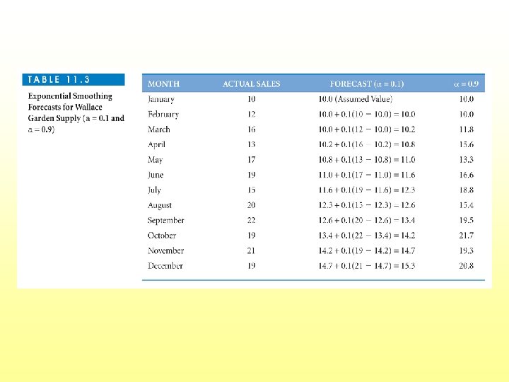
Wallace Garden Supply With Exponential Smoothing • Assume the smoothed value for the first month is the actual value • Use α = 0. 1 and also α = 0. 9

Trend Analysis • Fits a straight or curved line through a time series • We will cover only linear trends • A scatter diagram shows the trend • Excel can both create the scatter diagram and fit the linear trend line

Midwestern Electric Co. Example Go to file 11 -5. xls

The Trend Equation Ŷ = b 0 + b 1 X where, Ŷ = forecast average dependent value X = independent value (time) b 0 = Y-intercept b 1 = slope of the line

Least Squares Method The b 0 and b 1 values are found using the least squares method, which seeks to minimize the sum of squared errors SSE = ∑ (Y – Ŷ)2 Where, Error = Y - Ŷ

Least Squares Method for Best-Fitting Line

Least Squares Line With Excel • Can use regression in the Analysis Tool. Pak add-in • The time (X) values are transformed to 1, 2, 3, etc. Go to file 11 -6. xls

Seasonality Analysis • When a seasonal pattern repeats yearly, this can be used for future forecasts • Need monthly or quarterly data • A seasonal index is the ratio of the average value in that season, over the annual average

Eichler Supplies Seasonality Example • Have monthly demand data for 24 months • Calculate overall average monthly demand • Calculate ratio for each month Go to file 11 -7. xls

Decomposition of a Time Series • • Decomposition breaks a time series down into its components (Trend, Seasonal, Cyclical, and Random) Two types of models 1. Multiplicative 2. Additive

Multiplicative Decomposition Sawyer Piano House Example • • • Want to forecast sales of grand pianos Have quarterly data for the past 5 years Steps: 1. Find the seasonal indices • • First smooth data with moving averages Seasonal ratio = actual value / smoothed value Average the seasonal ratios for each quarter Unseasonalized value = actual value / seasonal index

Steps Continued 2. Find the trend equation using the unseasonalized values 3. Calculate forecasts • • Use the trend equation to make an unseasonalized forecast Multiply the unseasonalized forecast by the seasonal index 4. Calculate forecast error Go to file 11 -8. xls

Causal Forecasting Models • Forecasting a dependent variable based on other (independent) variables • Uses simple or multiple regression • Example: – Dependent variable: Swimwear sales – Independent variables: selling price, competitors prices, temperature, whether schools are in session, advertising

Causal Simple Regression Model • Want to predict selling price of homes (Y) based on the square footage (X) • Have data on 12 homes recently sold in a specific neighborhood • Use scatter diagram to check for linear relation • Find least squares equation Ŷ = b 0 + b 1 X

Causal Simple Regression With Excel. Modules Given the X and Y data, it will automatically: • Calculate the regression equation • Calculate forecast error • Produce a scatter plot with the regression line Go to file 11 -9. xls

The Regression Equation Forecast average selling price = -8. 125 + 97. 789(Home size) Slope interpretation: On average the price of a home will increase by $97. 789 thousand per additional thousand sq. ft. Intercept interpretation: When X=0 the average selling price is -$8. 125 thousand (has no practical meaning since no houses have 0 square feet)

Standard Error and Correlation • Standard Error (Sy, x) – the standard deviation of the regression equation (useful for confidence intervals on forecasts) • Correlation Coefficient (r) – measures the strength of the linear relation -1 < r < 1

Correlation Coefficient Examples

Coefficient of Determination (R 2) • Measures the proportion of variation in the dependent variable (Y) that can be explained with the independent variable (X) 0 < R 2 < 1 • It is the correlation squared

Using the Causal Simple Regression Model • To forecast the average selling price of a 3100 sq. foot home, use X = 3. 10 • Can use Excel. Modules to produce forecast • Forecast = -8. 125 + 97. 789(3. 1) = 295 which is $295, 000

Potential Weaknesses of Causal Forecasting With Regression • We need to provide the value(s) of the independent variable(s) • Individual values of Y may be much higher or lower than the forecast average • Model is generally valid only for X values within the range of the data set

Approximate Confidence Interval • Helpful for showing how high or low an individual value might be • Approximate confidence interval formula: Ŷ + Zα/2 (Sy, x) • Approximate 95% interval example: 295 + 1. 96 (42. 602) Which is $211, 500 to $378, 500

Causal Simple Regression Using Excel’s Analysis Tool. Pak • An add-in that includes regression • Appears as “Data Analysis” at the bottom of the “Tools” menu Go to file 11 -9. xls

Statistical Significance Tests • If the true value of the slope (β 1) does not differ significantly from 0, then Y does not change as X changes • Hypotheses: H 0: β 1=0 (X is not significantly related to Y) H 1: β 1≠ 0 (X is significantly related to Y) • Tested by both F-test and t-test • Reject H 0 if p-value < α

Hypothesis Test Results for Home Selling Prices From either F-test or t-test (they are equivalent for simple regression): Reject H 0 because p=0. 011 is < 0. 05 (alpha) Home size is statistically significant in having ability to predict home selling price

Causal Multiple Regression Model More than one independent variable Ŷ = b 0 + b 1 X 1 + b 2 X 2 + … + b p. X p Where, b 0 = Y-axis intercept (all X’s =0) bi = slope for Xi p = number of independent variables (X’s)

Causal Multiple Regression Using Excel’s Analysis Tool. Pak • All columns of independent variables must be adjacent to one another (no gaps) • The Analysis Tool. Pak add-in (Data Analysis) must be “turned on” Go to file 11 -10. xls

Statistical Significance Test Of the Overall Model (F-test) • If all true slope values (βi) equal 0, then the model has no ability to predict Y • Hypotheses: H 0: β 1=β 2=0 (model has no ability to predict Y) H 1: at least one βi ≠ 0 (at least one variable has ability to predict Y) • F-test is used

Statistical Significance Test of Individual Variables (t-test) • Tests whether an individual X is helping to predict Y (in the presence of the other X’s) • Hypotheses for each Xi: H 0: βi=0 (Xi adds no ability to predict Y, given the other X’s in the model) H 1: βi ≠ 0 (Xi adds ability to predict Y, given the other X’s in the model)

Hypothesis Test Results for Home Selling Prices • F-test: Overall model has significant ability to predict home prices • T-tests: Land area – is significant, given the presence of home size Home size – is not significant, given the presence of land area

Multicollinearity • Why did home size become nonsignificant when land area was added? • Multicollinearity exists when 2 or more independent variables are highly correlated • Correlations among X’s can be used to detect multicollinearity