Chapter 10 XML The world of XML

Chapter 10: XML The world of XML

Context • The dawn of database technology 70 s • A DBMS is a flexible store-recall system for digital information • It provides permanent memory for structured information

Context • Database Managements technology for administrative settings ‘completed’ in the early 80 s • Search for demanding application areas that could benefit from a database approach – A sound datamodel to structure the information and maintain integrity rules – A high level programming language model to manipulate the data – Separation of concerns between modelling and manipulation, and physical storage and order of execution thanks to query optimizer technology

Context • Demanding areas of research in DBMS core technology: – Office Information systems, e. g. document modelling and workflow – CAD/CAM, e. g. how to manage the design of an airplane or nucleur power plant – GIS, e. g. managing remote sensing information – WWW, e. g. how to integrate heterogenous sources – Agent-based systems, e. g. reactive systems – Multimedia, e. g. video storage/retrieval – Datamining, e. g. discovery of client profiles – Sensor networks, e. g. small footprint and energy-wise computing

Context • Demanding areas of research in DBMS core technology: – Office Information systems, Extensible DBMS, blobs – CAD/CAM, Object-oriented DBMS, geometry – GIS, GIS DBMS, geometry and images – Agent-based systems, Active DBMS, triggers – Multimedia, MM DBMS, feature analysis – Datamining, Datawarehouse systems, cube, association rules – Sensor networks, P 2 P databases, ad-hoc networking

Context • Application interaction with DBMS – Proprietary application programming interface, shielding the hardware distinctions – Use readable interfaces to improve monitoring and development • Example: in Monetdb the interaction is based on ascii text with the first character indicative for the message type ‘>’ prompt, await for next request ‘!’ error occurred, rest is the message ‘[‘ start of a tuple answer – Language embedding to remove the impedance mismatch, i. e. avoid cost of transforming data • Effectively failed in the OO world

Context • Learning points database perspective, – Database system should not be concerned with the userinteraction technology, ‘they should be blind and deaf’ – The strong requirements on schema, integrity rules and processing is a harness – Interaction with applications should be self-descriptive as much as possible, because, you can not a priori know a complete schema – Need for semi-structured databases

Semi-structured data • Properties of semistructured databases: – The schema is not given in advance and may be implicit in the data – The schema is relatively large and changes frequently – The schema is descriptive rather than prescriptive, integrity rules may be violated – The data is not strongly typed, the values of attributes may be of different type • Stanford Lore system is the prototypical first attempt to support semi-structured databases

Context Accidentally, in the world of digital publishing there is a need for a simple datamodel to structure information SMGL HTML XHTML XPATH XQUERY XSLT By the end 90 s, the document world meets the database world

Introduction • XML: Extensible Markup Language • Defined by the WWW Consortium (W 3 C) • Originally intended as a document markup language not a database language – Documents have tags giving extra information about sections of the document • E. g. Introduction … – Derived from SGML (Standard Generalized Markup Language), but simpler to use than SGML – Extensible, unlike HTML • Users can add new tags, and separately specify how the tag should be handled for display

XML Introduction (Cont. ) • The ability to specify new tags, and to create nested tag structures made XML a great way to exchange data, not just documents. – Much of the use of XML has been in data exchange applications, not as a replacement for HTML • Tags make data (relatively) self-documenting – E. g. A-101 Downtown 500 A-101 Johnson

XML: Motivation • Data interchange is critical in today’s networked world – Examples: • Banking: funds transfer • Order processing (especially inter-company orders) • Scientific data – Chemistry: Chem. ML, … – Genetics: BSML (Bio-Sequence Markup Language), … – Paper flow of information between organizations is being replaced by electronic flow of information • Each application area has its own set of standards for representing information (W 3 C maintains ca 30 standards) • XML has become the basis for all new generation data interchange formats

XML Motivation (Cont. ) • Each XML based standard defines what are valid elements, using – XML type specification languages to specify the syntax • DTD (Document Type Descriptors) • XML Schema – Plus textual descriptions of the semantics • XML allows new tags to be defined as required – However, this may be constrained by DTDs • A wide variety of tools is available for parsing, browsing and querying XML documents/data

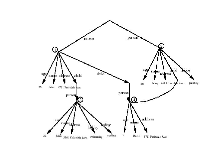
Motivation for Nesting • Nesting of data is useful in data transfer – Example: elements representing customer-id, customer name, and address nested within an order element • Nesting is not supported, or discouraged, in relational databases – With multiple orders, customer name and address are stored redundantly – normalization replaces nested structures in each order by foreign key into table storing customer name and address information – Nesting is supported in object-relational databases and NF 2 • But nesting is appropriate when transferring data – External application does not have direct access to data referenced by a foreign key

Example of Nested Elements Hayes Main Harrison A-102 Perryridge 400 … . .

Structure of XML Data (Cont. ) • Mixture of text with sub-elements is legal in XML. – Example: This account is seldom used any more. A-102 Perryridge 400 – Useful for document markup, but discouraged for data representation

Attributes • Elements can have attributes – A-102 Perryridge 400 • Attributes are specified by name=value pairs inside the starting tag of an element • An element may have several attributes, but each attribute name can only occur once •

Attributes Vs. Subelements • Distinction between subelement and attribute – In the context of documents, attributes are part of markup, while subelement contents are part of the basic document contents – In the context of data representation, the difference is unclear and may be confusing • Same information can be represented in two ways – …. – A-101 … – Suggestion: use attributes for identifiers of elements, and use subelements for contents

XML Document Schema • Database schemas constrain what information can be stored, and the data types of stored values • XML documents are not required to have an associated schema • However, schemas are very important for XML data exchange – Otherwise, a site cannot automatically interpret data received from another site • Two mechanisms for specifying XML schema – Document Type Definition (DTD) • Widely used – XML Schema • Newer, not yet widely used

Attribute Specification in DTD • Attribute specification : for each attribute – Name – Type of attribute • CDATA • ID (identifier) or IDREF (ID reference) or IDREFS (multiple IDREFs) – more on this later – Whether • mandatory (#REQUIRED) • has a default value (value), • or neither (#IMPLIED) • Examples – –

IDs and IDREFs • An element can have at most one attribute of type ID • The ID attribute value of each element in an XML document must be distinct – Thus the ID attribute value is an object identifier • An attribute of type IDREF must contain the ID value of an element in the same document • An attribute of type IDREFS contains a set of (0 or more) ID values. Each ID value must contain the ID value of an element in the same document

Limitations of DTDs • No typing of text elements and attributes – All values are strings, no integers, reals, etc. • Difficult to specify unordered sets of subelements – Order is usually irrelevant in databases – (A | B)* allows specification of an unordered set, but • Cannot ensure that each of A and B occurs only once • IDs and IDREFs are untyped – The owners attribute of an account may contain a reference to another account, which is meaningless • owners attribute should ideally be constrained to refer to customer elements

XML Schema • XML Schema is a more sophisticated schema language which addresses the drawbacks of DTDs. Supports – Typing of values • E. g. integer, string, etc • Also, constraints on min/max values – User defined types – Is itself specified in XML syntax, unlike DTDs • More standard representation, but verbose – Is integrated with namespaces – Many more features • List types, uniqueness and foreign key constraints, inheritance. . • BUT: significantly more complicated than DTDs, not yet widely used.

Storage of XML Data • XML data can be stored in – Non-relational data stores • Flat files – Natural for storing XML – But has all problems discussed in Chapter 1 (no concurrency, no recovery, …) • XML database – Database built specifically for storing XML data, supporting DOM model and declarative querying – Currently no commercial-grade scaleable system – Relational databases • Data must be translated into relational form • Advantage: mature database systems • Disadvantages: overhead of translating data and queries

Storing XML in Relational Databases • Store as string – E. g. store each top level element as a string field of a tuple in a database • Use a single relation to store all elements, or • Use a separate relation for each top-level element type – E. g. account, customer, depositor – Indexing: » Store values of subelements/attributes to be indexed, such as customer-name and account-number as extra fields of the relation, and build indices » Oracle 9 supports function indices which use the result of a function as the key value. Here, the function should return the value of the required subelement/attribute » SQL server 2005 same

Storing XML in Relational Databases • Store as string – E. g. store each top level element as a string field of a tuple in a database – Benefits: • Can store any XML data even without DTD • As long as there are many top-level elements in a document, strings are small compared to full document, allowing faster access to individual elements. – Drawback: Need to parse strings to access values inside the elements; parsing is slow.

OEM model • Semi structured and XML databases can be modelled as graph-problems • Early prototypes directly supported the graph model as the physical implementation scheme. Querying the graph model was implemented using graph traversals • XML without IDREFS can be modelled as trees

Storing XML as Relations (Cont. ) • Tree representation: model XML data as tree and store using relations nodes(id, type, label, value) child (child-id, parent-id) – Each element/attribute is given a unique identifier – Type indicates element/attribute – Label specifies the tag name of the element/name of attribute – Value is the text value of the element/attribute – The relation child notes the parent-child relationships in the tree • Can add an extra attribute to child to record ordering of children – Benefit: Can store any XML data, even without DTD – Drawbacks: • Data is broken up into too many pieces, increasing space overheads • Even simple queries require a large number of joins, which can be slow

Storing XML in Relations (Cont. ) • Map to relations • If DTD of document is known, you can map data to relations – Bottom-level elements and attributes are mapped to attributes of relations – A relation is created for each element type • An id attribute to store a unique id for each element • all element attributes become relation attributes • All subelements that occur only once become attributes – For text-valued subelements, store the text as attribute value – For complex subelements, store the id of the subelement • Subelements that can occur multiple times represented in a separate table – Similar to handling of multivalued attributes when converting ER diagrams to tables – Benefits: • Efficient storage • Can translate XML queries into SQL, execute efficiently, and then translate SQL results back to XML

Alternative mappings • Mapping the structure – The Edge approach – The Attribute approach – The Universal Table approach – The Normalized Universal approach – The Dataguide approach • Mapping values – Separate value tables – Inlining • Shredding

Edge approach • Use a single Edge table to capture the graph structure Edge(source, ordinal, name, flag, target) Flag: {value, reference} Keys: {source, ordinal) Index: source, {name, target}

Attribute approach • Group all attributes with the same name into one table Aname(source, ordinal, flag, target) Key: {source, ordinal} Index: {target}

Universal approach • Use the Universal Table, all attributes are stored as columns Universal(source, ord-1, flag-1, target-1, …, ord-n, flag-n, target-n) Key: source, index: target-i

Normalized Universal • Same as Universal, but factor out the repeating values Universal(source, ord-1, flag-1, target-1, …, ord-n, flag-n, target-n) Overflow_n(source, ord, flag, target) Key: source, and {source, ord} Index: target-i

Mapping values • Separate value tables – Use V_type(vid, value) tables, eg. int(vid, val), str(vid, val), ….

Mapping values • Inlining – As illustrated in previous mappings, inline the values in the structure relations

Shredding • Try to recognize repeating structures and map them to separate tables • Handle the remainder through any of the previous methods

Evaluation • Some results reported by Florescu, Kossmann using a commercial DBMS on documents of 100 K objects in 1999 • Database storage overhead:

Evaluation • Some results reported by Florescu, Kossmann using a commercial DBMS on documents of 100 K objects in 1999 • Bulk loading:

Evaluation • Some results reported by Florescu, Kossmann using a commercial DBMS on documents of 100 K objects in 1999 • Reconstruction:

The Data Semistructured data instance = a large graph

The indexing problem • The storage problem – Store the graph in a relational DBMS – Develop a new database storage structure • The indexing problem: – Input: large, irregular data graph – Output: index structure for evaluating (regular) path expressions, e. g. bib. paper. author. firstname

XSet: a simple index for XML • Part of the Ninja project at Berkeley • Example XML data:

XSet: a simple index for XML Each node = a hashtable Each entry = list of pointers to data nodes (not shown)

XSet: Efficient query evaluation • • SELECT X X FROM part. name X part. supplier. name X part. *. subpart. name X *. supplier. name X Will gain when index fits in memory -yes -maybe

Region Algebras • structured text = text with tags (like XML) • data = sequence of characters [c 1 c 2 c 3 …] • region = interval in the text – representation (x, y) = [cx, cx+1, … cy] – example:

Region algebra: some operators • s 1 intersect s 2 = {r | r s 1, r s 2} • s 1 included s 2 = {r | r s 1, r’ s 2, r r’} • s 1 including s 2 = {r | r s 1, r’ s 2, r r’} • s 1 parent s 2 = {r | r s 1, r’ s 2, r is a parent of r’} • s 1 child s 2 = {r | r s 1, r’ s 2, r is child of r’} Examples: included including

Efficient computation of Region Algebra Operators Example: s 1 included s 2 s 1 = {(x 1, x 1'), (x 2, x 2'), …} s 2 = {(y 1, y 1'), (y 2, y 2'), …} (i. e. assume each consists of disjoint regions) Algorithm: if xi < yj then i : = i + 1 if xi' > yj' then j : = j + 1 otherwise: print (xi, xi'), do i : = i + 1 Can do in sub-linear time when one region is very small

From path expressions to region expressions Region expressions correspond to simple XPath expressions part. name part. supplier. name *. supplier. name part. *. subpart. name child (part child root) name child (supplier child (part child root)) name child supplier name child (subpart included (part child root))

Storage structures for region algebras • Every node is characterised by an integer pair (x, y) • This means we have a 2 -d space • Any 2 -d space data structure can be used • If you use a (pre-order, post-order) numbering you get triangular filling of 2 -d (to be discussed later)

Alternative mappings • Mapping the structure to the relational world – The Edge approach – The Attribute approach – The Universal Table approach – The Normalized Universal approach – The Monet/XML approach – The Dataguide approach • Mapping values – Separate value tables – Inlining • Shredding

Dataguide approach • Developed in the context of Lore, Lorel (Stanford Univ) • Predecessor of the Monet/XML model • Observation: – queries in the graph-representation take a limited form – they are partial walks from the root to an object of interest – this behaviour was stressed by the query language Lorel, i. e. an SQL-based query language based on processing regular expressions SELECT X FROM (Bib. *. author). (lastname|firstname). Abiteboul X

Data. Guides Definition given a semistructured data instance DB, a Data. Guide for DB is a graph G s. t. : - every path in DB also occurs in G - every path in G occurs in DB - every path in G is unique

Dataguides Example:

Data. Guides • Multiple Data. Guides for the same data:

Data. Guides Definition Let w, w’ be two words (I. e word queries) and G a graph w G w’ if w(G) = w’(G) Definition G is a strong dataguide for a database DB if G is the same as DB Example: - G 1 is a strong dataguide - G 2 is not strong person. project ! DB dept. project person. project ! G 2 dept. project

Data. Guides • Constructing the strong Data. Guide G: Nodes(G)={{root}} Edges(G)= while changes do choose s in Nodes(G), a in Labels add s’={y|x in s, (x -a->y) in Edges(DB)} to Nodes(G) add (x -a->y) to Edges(G) • Use hash table for Nodes(G) • This is precisely the powerset automaton construction.

Data. Guides • How large are the dataguides ? – if DB is a tree, then size(G) <= size(DB) • why? answer: every node is in exactly one extent of G • here: dataguide = XSet – How many nodes does the strong dataguide have for this DB ? 20 nodes (least common multiple of 4 and 5) Dataguides usually fail on data with cyclic schemas, like: