bc1243ad3adc0c5ec990a4a21ce1bd94.ppt
- Количество слайдов: 116

Chapter 10 THE PARTIAL EQUILIBRIUM COMPETITIVE MODEL: -Market demand -Market supply Copyright © 2005 by South-Western, a division of Thomson Learning. All rights reserved. 1

Market Demand We start by studying the demand of the market 2
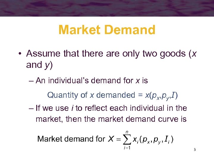
Market Demand • Assume that there are only two goods (x and y) – An individual’s demand for x is Quantity of x demanded = x(px, py, I) – If we use i to reflect each individual in the market, then the market demand curve is 3
Market Demand • To construct the market demand curve, PX is allowed to vary while Py and the income of each individual are held constant • If each individual’s demand for x is downward sloping, the market demand curve will also be downward sloping 4
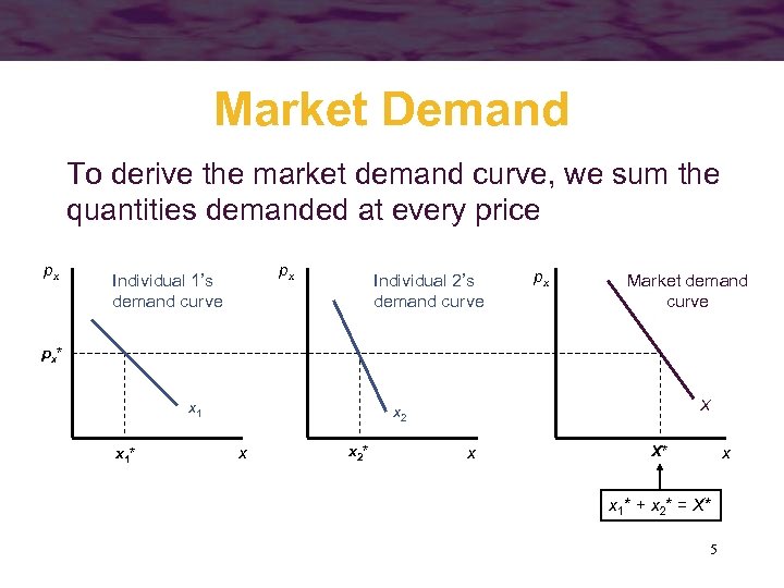
Market Demand To derive the market demand curve, we sum the quantities demanded at every price px px Individual 1’s demand curve Individual 2’s demand curve px Market demand curve px* x 1* X x 2 x x 2* x X* x x 1* + x 2* = X* 5
Shifts in the Market Demand Curve • The market demand summarizes the ceteris paribus relationship between X and px – changes in px result in movements along the curve (change in quantity demanded) – changes in other determinants of the demand for X cause the demand curve to shift to a new position (change in demand) – See example 10. 1 in the book to see how to do it mathematically 6
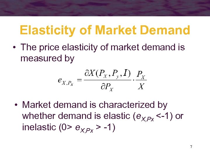
Elasticity of Market Demand • The price elasticity of market demand is measured by • Market demand is characterized by whether demand is elastic (e. X, Px <-1) or inelastic (0> e. X, Px > -1) 7
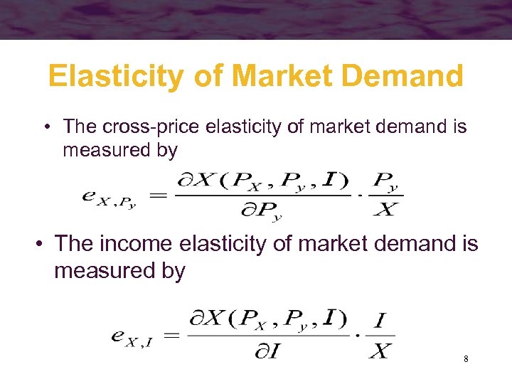
Elasticity of Market Demand • The cross-price elasticity of market demand is measured by • The income elasticity of market demand is measured by 8

• We will study supply of the market and the market equilibrium • The way the equilibrium is determined depends on whether we are studying short run, or long run • From the time being, we will focus our attention on studying the equilibrium in perfectly competitive industries 9
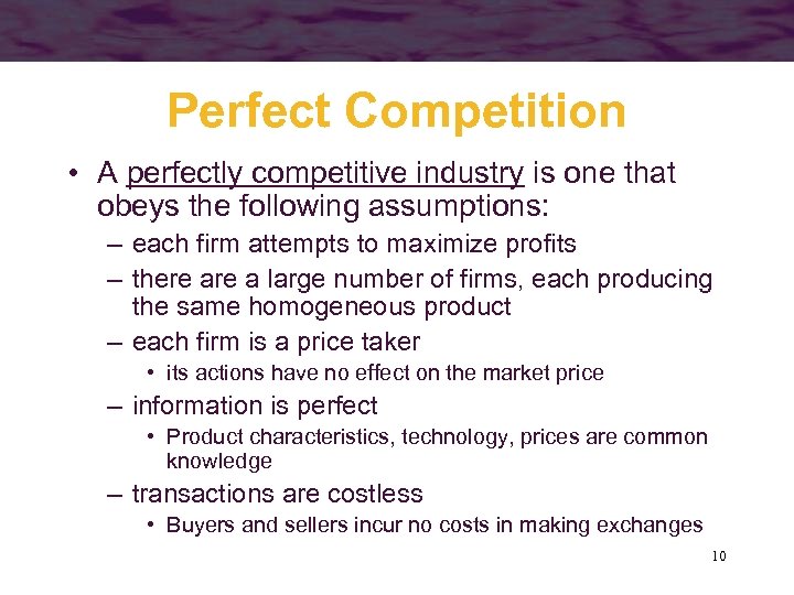
Perfect Competition • A perfectly competitive industry is one that obeys the following assumptions: – each firm attempts to maximize profits – there a large number of firms, each producing the same homogeneous product – each firm is a price taker • its actions have no effect on the market price – information is perfect • Product characteristics, technology, prices are common knowledge – transactions are costless • Buyers and sellers incur no costs in making exchanges 10
Timing of the Supply Response • In the analysis of competitive pricing, the time period under consideration is important • The time period will be important to determine the supply curve – very short run (not very interesting, we will not study it…) – short run • existing firms can alter their quantity supplied by altering the quantity of the variable input (labour), but quantity of fixed inputs cannot be changed, hence no new firms can enter the industry – long run • new firms may enter an industry 11
Market Supply in the short run • The quantity of output supplied to the entire market in the short run is the sum of the quantities supplied by each firm – the amount supplied by each firm depends on price • The short-run market supply curve will be upward-sloping because each firm’s short-run supply curve has a positive slope 12
Determination of the eq. Price in the short run • The number of firms in an industry is fixed • These firms are able to adjust the quantity they are producing – they can do this by altering the levels of the variable inputs they employ 13
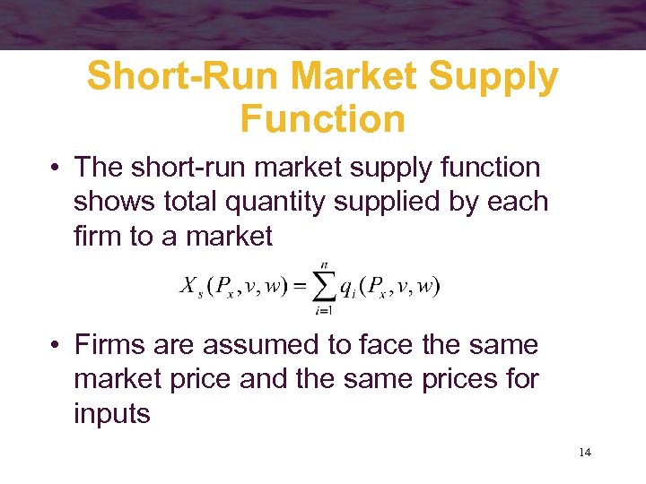
Short-Run Market Supply Function • The short-run market supply function shows total quantity supplied by each firm to a market • Firms are assumed to face the same market price and the same prices for inputs 14
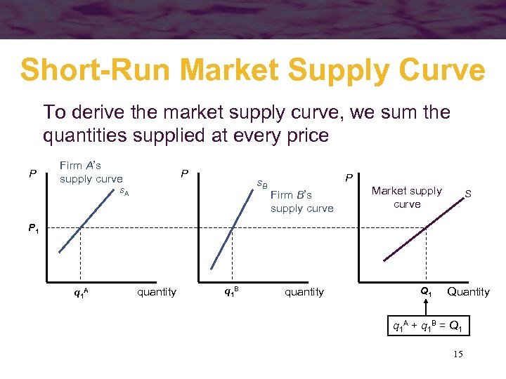
Short-Run Market Supply Curve To derive the market supply curve, we sum the quantities supplied at every price P Firm A’s supply curve P s. B s. A P Firm B’s supply curve Market supply curve S P 1 q 1 A quantity q 1 B quantity Q 1 Quantity q 1 A + q 1 B = Q 1 15
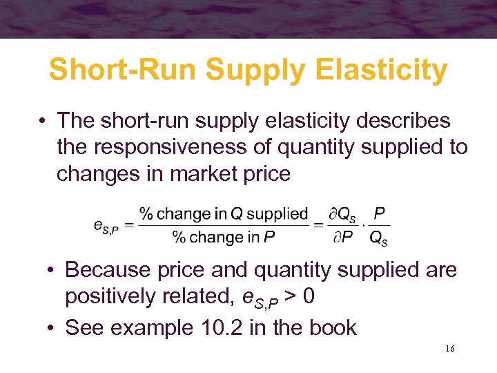
Short-Run Supply Elasticity • The short-run supply elasticity describes the responsiveness of quantity supplied to changes in market price • Because price and quantity supplied are positively related, e. S, P > 0 • See example 10. 2 in the book 16
Equilibrium Price Determination in the SR • We have studied the market demand • We have studied the short run supply curve • So, we can study the short run market equilibrium 17
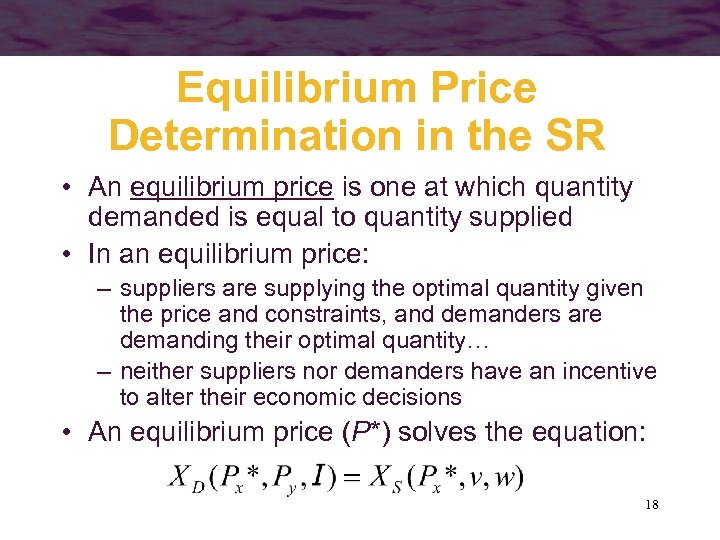
Equilibrium Price Determination in the SR • An equilibrium price is one at which quantity demanded is equal to quantity supplied • In an equilibrium price: – suppliers are supplying the optimal quantity given the price and constraints, and demanders are demanding their optimal quantity… – neither suppliers nor demanders have an incentive to alter their economic decisions • An equilibrium price (P*) solves the equation: 18

Equilibrium Price Determination • The equilibrium price depends on many exogenous factors: – Demand curves depend on other goods prices, income, preferences (utility function) – Supply curves depend on inputs prices – changes in any of these factors will likely result in a new equilibrium price • Economists predict the new situation by computing the new equilibrium. The equilibrium is an economist’s prediction of the new situation after a change has taken place 19
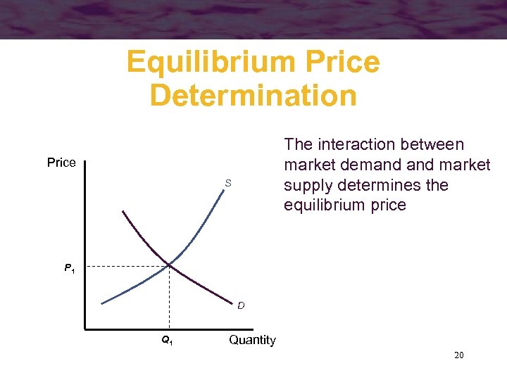
Equilibrium Price Determination The interaction between market demand market supply determines the equilibrium price Price S P 1 D Q 1 Quantity 20
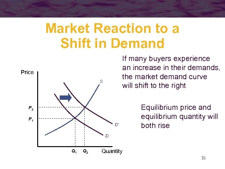
Market Reaction to a Shift in Demand If many buyers experience an increase in their demands, the market demand curve will shift to the right Price S P 2 P 1 D’ Equilibrium price and equilibrium quantity will both rise D Q 1 Q 2 Quantity 21
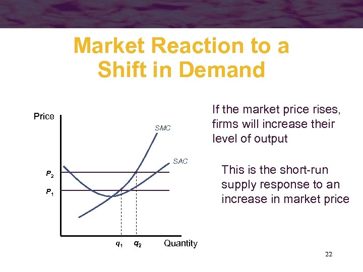
Market Reaction to a Shift in Demand If the market price rises, firms will increase their level of output Price SMC SAC P 2 P 1 q 2 This is the short-run supply response to an increase in market price Quantity 22
Shifts in Supply and Demand Curves • Demand curves shift because – incomes change – prices of substitutes or complements change – preferences change • Supply curves shift because – input prices change – technology changes – number of producers change 23
Shifts in Supply and Demand Curves • When either a supply curve or a demand curve shift, equilibrium price and quantity will change • The relative magnitudes of these changes depends on the shapes of the supply and demand curves (elasticity is very important !!!!) • See example 10. 3 in the book 24
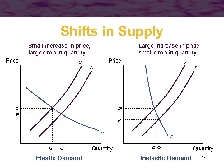
Shifts in Supply Small increase in price, large drop in quantity Price Large increase in price, small drop in quantity Price S’ S’ S S P’ P D D Q’ Q Elastic Demand Quantity Q’ Q Inelastic Demand Quantity 25
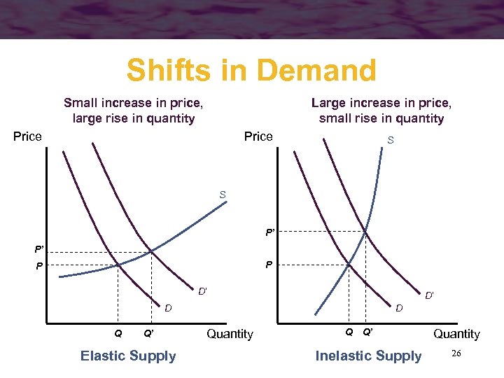
Shifts in Demand Small increase in price, large rise in quantity Large increase in price, small rise in quantity Price S S P’ P’ P P D’ D’ D Q Q’ Elastic Supply D Quantity Q Q’ Quantity Inelastic Supply 26

Putting it together… • Using econometrics, we can estimate the demand supply curve, and how they depend on other factors (input prices, other goods’ prices…) • Compute the new equilibrium when these other factors change • This would be our prediction… • However, it could be enough to estimate the different elasticities rather than the whole new curves 27
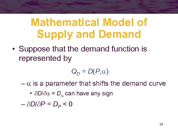
Mathematical Model of Supply and Demand • Suppose that the demand function is represented by QD = D(P, ) – is a parameter that shifts the demand curve • D/ = D can have any sign – D/ P = DP < 0 28
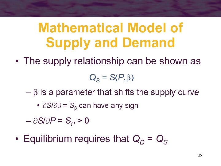
Mathematical Model of Supply and Demand • The supply relationship can be shown as QS = S(P, ) – is a parameter that shifts the supply curve • S/ = S can have any sign – S/ P = SP > 0 • Equilibrium requires that QD = QS 29
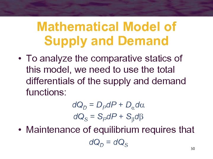
Mathematical Model of Supply and Demand • To analyze the comparative statics of this model, we need to use the total differentials of the supply and demand functions: d. QD = DPd. P + D d d. QS = SPd. P + S d • Maintenance of equilibrium requires that d. QD = d. QS 30
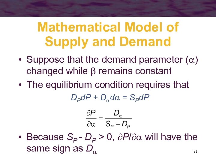
Mathematical Model of Supply and Demand • Suppose that the demand parameter ( ) changed while remains constant • The equilibrium condition requires that DPd. P + D d = SPd. P • Because SP - DP > 0, P/ will have the same sign as D 31
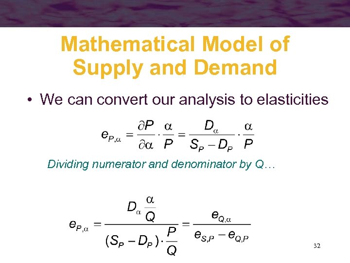
Mathematical Model of Supply and Demand • We can convert our analysis to elasticities Dividing numerator and denominator by Q… 32
Long-Run Analysis • So far, we have studied short run… • In the long run, a firm may adapt all of its inputs to fit market conditions – profit-maximization for a price-taking firm implies that price is equal to long-run MC • Firms can also enter and exit an industry in the long run – perfect competition assumes that there are no special costs of entering or exiting an industry 33
Long-Run Analysis • New firms will be lured into any market for which economic profits are greater than zero – entry of firms will cause the short-run industry supply curve to shift outward – market price and profits will fall – the process will continue until economic profits are zero 34
Long-Run Analysis • Existing firms will leave any industry for which economic profits are negative – exit of firms will cause the short-run industry supply curve to shift inward – market price will rise and losses will fall – the process will continue until economic profits are zero 35
Long-Run Competitive Equilibrium • A perfectly competitive industry is in long-run equilibrium if there are no incentives for profit-maximizing firms to enter or to leave the industry – That is, if profits are zero in the longrun equilibrium – this will occur when the number of firms is such that P = MC = AC and each firm operates at minimum AC 36

Long-Run Competitive Equilibrium • We will assume that all firms in an industry have identical cost curves – no firm controls any special resources or technology • The equilibrium long-run position requires that each firm earn zero economic profit 37
Long-Run Equilibrium: Constant-Cost Case • Assume that the entry of new firms in an industry has no effect on the cost of inputs – no matter how many firms enter or leave an industry, a firm’s cost curves will remain unchanged • This is referred to as a constant-cost industry (Example 10. 5) 38
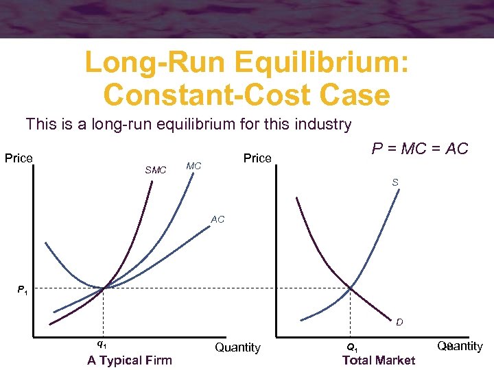
Long-Run Equilibrium: Constant-Cost Case This is a long-run equilibrium for this industry Price SMC P = MC = AC Price MC S AC P 1 D q 1 A Typical Firm Quantity Q 1 Total Market 39 Quantity
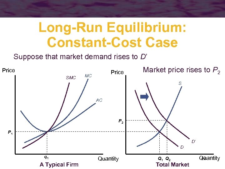
Long-Run Equilibrium: Constant-Cost Case Suppose that market demand rises to D’ Price SMC Price MC Market price rises to P 2 S AC P 2 P 1 D’ D q 1 A Typical Firm Quantity Q 1 Q 2 Total Market 40 Quantity
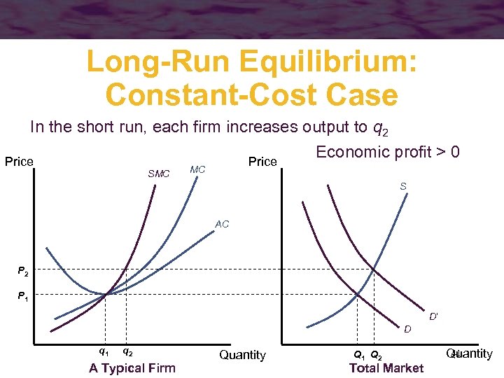
Long-Run Equilibrium: Constant-Cost Case In the short run, each firm increases output to q 2 Economic profit > 0 Price SMC Price MC S AC P 2 P 1 D’ D q 1 q 2 A Typical Firm Quantity Q 1 Q 2 Total Market 41 Quantity
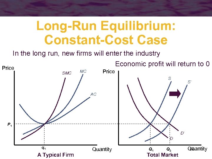
Long-Run Equilibrium: Constant-Cost Case In the long run, new firms will enter the industry Economic profit will return to 0 Price SMC Price MC S S’ AC P 1 D’ D q 1 A Typical Firm Quantity Q 1 Q 3 Total Market 42 Quantity
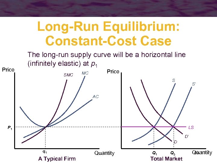
Long-Run Equilibrium: Constant-Cost Case Price The long-run supply curve will be a horizontal line (infinitely elastic) at p 1 SMC Price MC S S’ AC P 1 LS D’ D q 1 A Typical Firm Quantity Q 1 Q 3 Total Market 43 Quantity
Shape of the Long-Run Supply Curve • The zero-profit condition is the factor that determines the shape of the long-run cost curve – if average costs are constant as firms enter, long-run supply will be horizontal – if average costs rise as firms enter, long-run supply will have an upward slope – if average costs fall as firms enter, long-run supply will be negatively sloped 44
Long-Run Equilibrium: Increasing-Cost Industry • The entry of new firms may cause the average costs of all firms to rise – prices of scarce inputs may rise – new firms may impose “external” costs on existing firms – new firms may increase the demand for tax -financed services 45
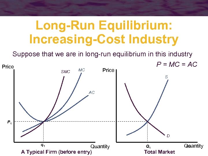
Long-Run Equilibrium: Increasing-Cost Industry Suppose that we are in long-run equilibrium in this industry P = MC = AC Price SMC Price MC S AC P 1 D q 1 Quantity A Typical Firm (before entry) Q 1 Total Market 46 Quantity
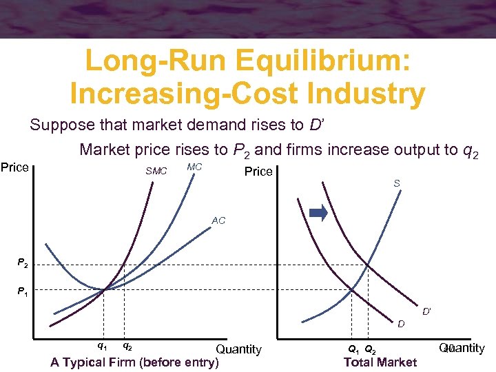
Long-Run Equilibrium: Increasing-Cost Industry Price Suppose that market demand rises to D’ Market price rises to P 2 and firms increase output to q 2 SMC MC Price S AC P 2 P 1 D’ D q 1 q 2 Quantity A Typical Firm (before entry) Q 1 Q 2 Total Market 47 Quantity
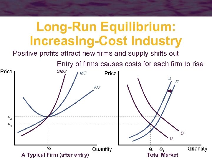
Long-Run Equilibrium: Increasing-Cost Industry Positive profits attract new firms and supply shifts out Entry of firms causes costs for each firm to rise Price SMC’ Price MC’ S S’ AC’ P 3 P 1 D’ D q 3 A Typical Firm (after entry) Quantity Q 1 Q 3 Total Market 48 Quantity
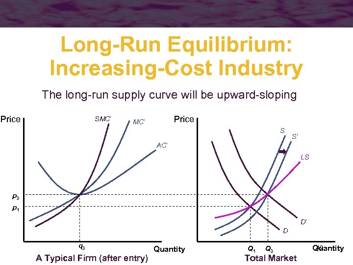
Long-Run Equilibrium: Increasing-Cost Industry The long-run supply curve will be upward-sloping Price SMC’ Price MC’ S S’ AC’ LS p 3 p 1 D’ D q 3 A Typical Firm (after entry) Quantity Q 1 Q 3 Total Market 49 Quantity
Long-Run Equilibrium: Decreasing-Cost Industry • The entry of new firms may cause the average costs of all firms to fall – new firms may attract a larger pool of trained labor – entry of new firms may provide a “critical mass” of industrialization • permits the development of more efficient transportation and communications networks 50
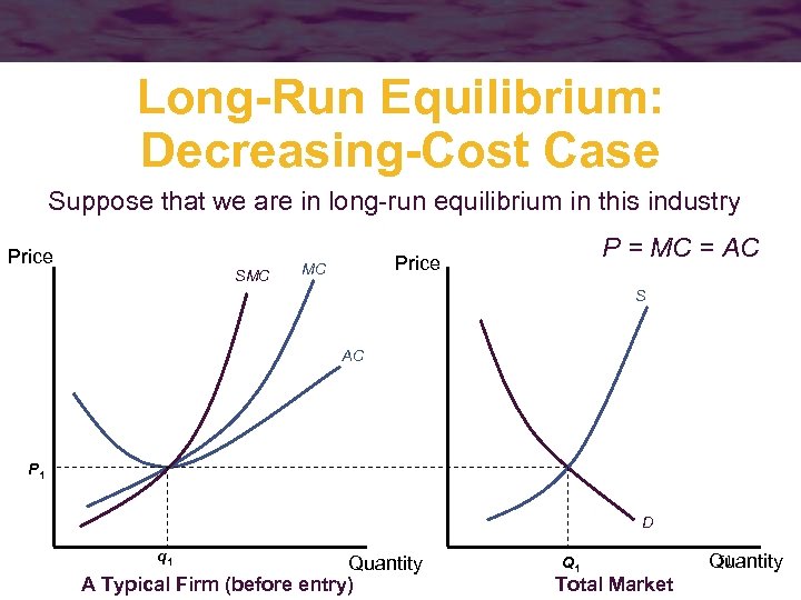
Long-Run Equilibrium: Decreasing-Cost Case Suppose that we are in long-run equilibrium in this industry Price SMC P = MC = AC Price MC S AC P 1 D q 1 Quantity A Typical Firm (before entry) Q 1 Total Market 51 Quantity
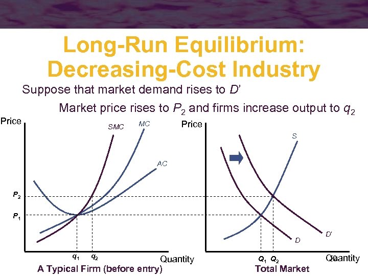
Long-Run Equilibrium: Decreasing-Cost Industry Price Suppose that market demand rises to D’ Market price rises to P 2 and firms increase output to q 2 SMC Price MC S AC P 2 P 1 D q 1 q 2 Quantity A Typical Firm (before entry) Q 1 Q 2 Total Market D’ 52 Quantity
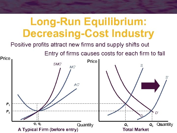
Long-Run Equilibrium: Decreasing-Cost Industry Price Positive profits attract new firms and supply shifts out Entry of firms causes costs for each firm to fall SMC’ Price S MC’ S’ AC’ P 1 P 3 D’ D q 1 q 3 Quantity A Typical Firm (before entry) Q 1 Total Market Q 3 53 Quantity
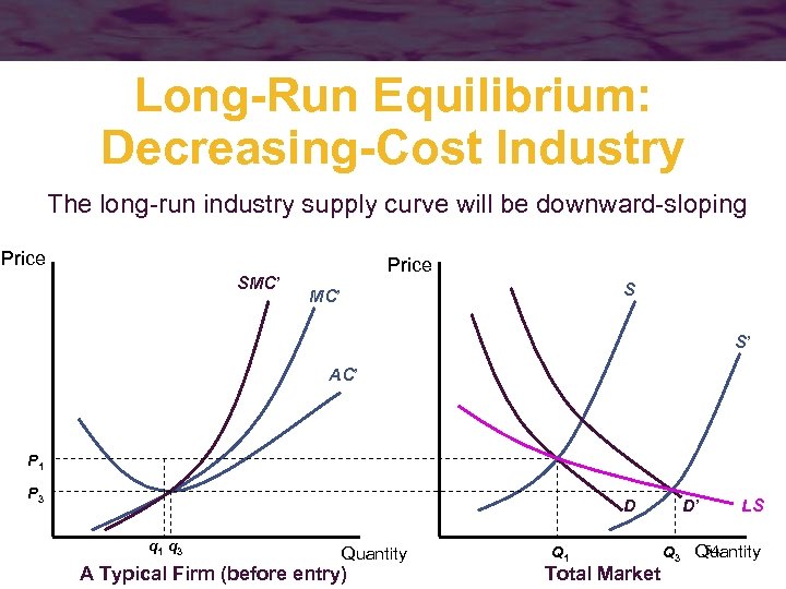
Long-Run Equilibrium: Decreasing-Cost Industry The long-run industry supply curve will be downward-sloping Price SMC’ Price S MC’ S’ AC’ P 1 P 3 D q 1 q 3 Quantity A Typical Firm (before entry) Q 1 Total Market D’ LS 54 Q 3 Quantity
Classification of Long-Run Supply Curves • Constant Cost – entry does not affect input costs – the long-run supply curve is horizontal at the long-run equilibrium price • Increasing Cost – entry increases inputs costs – the long-run supply curve is positively sloped 55
Classification of Long-Run Supply Curves • Decreasing Cost – entry reduces input costs – the long-run supply curve is negatively sloped 56
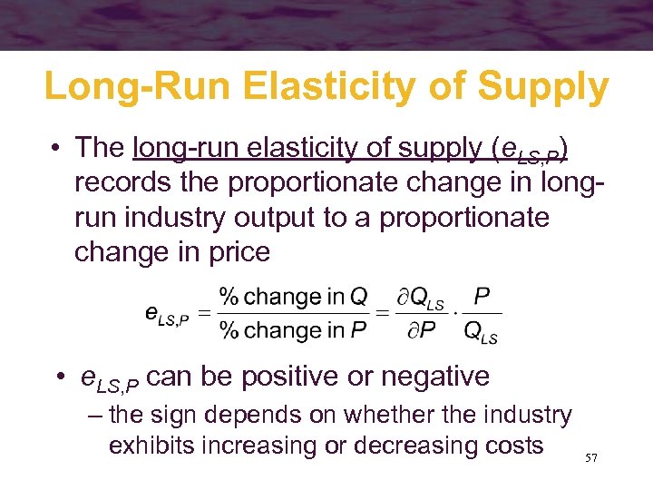
Long-Run Elasticity of Supply • The long-run elasticity of supply (e. LS, P) records the proportionate change in longrun industry output to a proportionate change in price • e. LS, P can be positive or negative – the sign depends on whether the industry exhibits increasing or decreasing costs 57
Comparative Statics Analysis of Long-Run Equilibrium • Comparative statics analysis of long-run equilibria can be conducted using estimates of long-run elasticities of supply and demand • Remember that, in the long run, the number of firms in the industry will vary from one long-run equilibrium to another 58
Comparative Statics Analysis of Long-Run Equilibrium • Assume that we are examining a constant-cost industry • Suppose that the initial long-run equilibrium industry output is Q 0 and the typical firm’s output is q* (where AC is minimized) • The equilibrium number of firms in the industry (n 0) is Q 0/q* 59
Comparative Statics Analysis of Long-Run Equilibrium • A shift in demand that changes the equilibrium industry output to Q 1 will change the equilibrium number of firms to n 1 = Q 1/q* • The change in the number of firms is – completely determined by the extent of the demand shift and the optimal output level for 60 the typical firm
Comparative Statics Analysis of Long-Run Equilibrium • The effect of a change in input prices can also be studied – See example 10. 6 in the book 61
Important Points to Note: • In the short run, equilibrium prices are established by the intersection of what demanders are willing to pay (as reflected by the demand curve) and what firms are willing to produce (as reflected by the short-run supply curve) – these prices are treated as fixed in both demanders’ and suppliers’ decision-making processes 62
Important Points to Note: • A shift in either demand or supply will cause the equilibrium price to change – the extent of such a change will depend on the slopes of the various curves • Firms may earn positive profits in the short run – because fixed costs must always be paid, firms will choose a positive output as long as revenues exceed variable costs 63

Important Points to Note: • In the long run, the number of firms is variable in response to profit opportunities – the assumption of free entry and exit implies that firms in a competitive industry will earn zero economic profits in the long run (P = AC) – because firms also seek maximum profits, the equality P = AC = MC implies that firms will operate at the low points of their long-run average cost curves 64
Important Points to Note: • The shape of the long-run supply curve depends on how entry and exit affect firms’ input costs – in the constant-cost case, input prices do not change and the long-run supply curve is horizontal – if entry raises input costs, the long-run supply curve will have a positive slope 65

Important Points to Note: • Changes in long-run market equilibrium will also change the number of firms – precise predictions about the extent of these changes is made difficult by the possibility that the minimum average cost level of output may be affected by changes in input costs or by technical progress 66
Important Points to Note: • If changes in the long-run equilibrium in a market change the prices of inputs to that market, the welfare of the suppliers of these inputs will be affected – such changes can be measured by changes in the value of long-run producer surplus 67

Chapter 11 APPLIED COMPETITIVE ANALYSIS Copyright © 2005 by South-Western, a division of Thomson Learning. All rights reserved. 68

Economic Efficiency and Welfare Analysis • The area between the demand the supply curve represents the sum of consumer and producer surplus – measures the total additional value obtained by market participants by being able to make market transactions • This area is maximized at the competitive market equilibrium 69
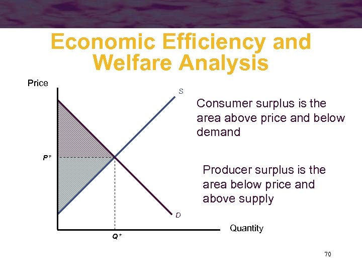
Economic Efficiency and Welfare Analysis Price S Consumer surplus is the area above price and below demand P* Producer surplus is the area below price and above supply D Q* Quantity 70
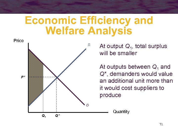
Economic Efficiency and Welfare Analysis Price S At output Q 1, total surplus will be smaller At outputs between Q 1 and Q*, demanders would value an additional unit more than it would cost suppliers to produce P* D Q 1 Q* Quantity 71

Economic Efficiency and Welfare Analysis • This tell us that under the assumptions that we have used (competitive industry), the government must argue why she was to alter the equilibrium price through policy 72
Welfare Loss Computations • Use of consumer and producer surplus notions makes possible the explicit calculation of welfare losses caused by restrictions on voluntary transactions – in the case of linear demand supply curves, the calculation is simple because the areas of loss are often triangular 73
Welfare Loss Computations • Suppose that the demand is given by QD = 10 - P and supply is given by QS = P - 2 • Market equilibrium occurs where P* = 6 and Q* = 4 74
Welfare Loss Computations • Restriction of output to Q 0 = 3 would create a gap between what demanders are willing to pay (PD) and what suppliers require (PS) PD = 10 - 3 = 7 PS = 2 + 3 = 5 75
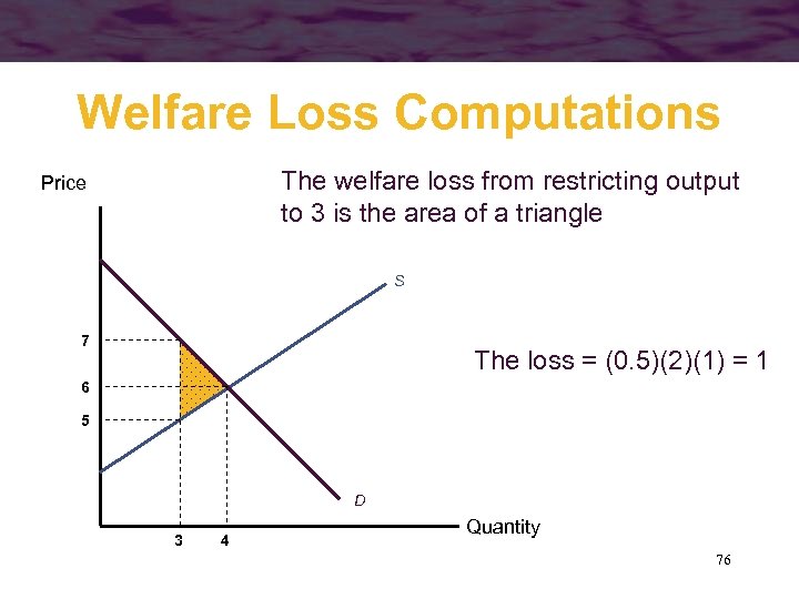
Welfare Loss Computations The welfare loss from restricting output to 3 is the area of a triangle Price S 7 The loss = (0. 5)(2)(1) = 1 6 5 D 3 4 Quantity 76
Welfare Loss Computations • The welfare loss will be shared by producers and consumers • In general, it will depend on the price elasticity of demand the price elasticity of supply to determine who bears the larger portion of the loss – the side of the market with the smallest price elasticity (in absolute value) 77

Price Controls and Shortages • Sometimes governments may seek to control prices at below equilibrium levels – this will lead to a shortage • We can look at the changes in producer and consumer surplus from this policy to analyze its impact on welfare 78
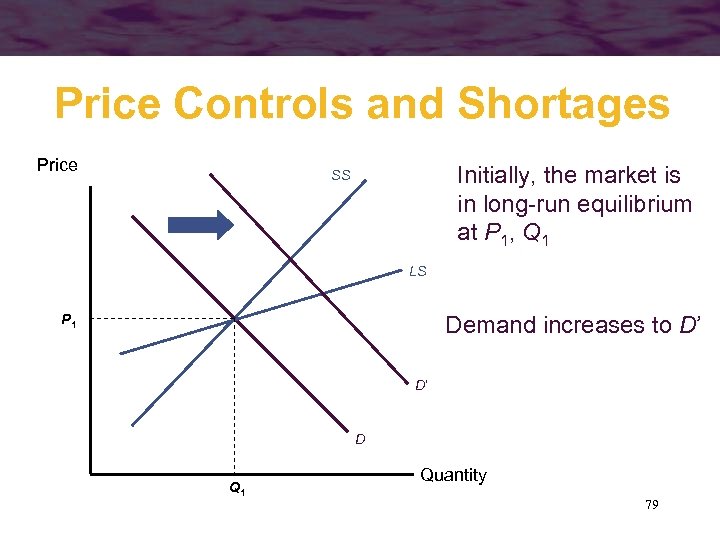
Price Controls and Shortages Price Initially, the market is in long-run equilibrium at P 1, Q 1 SS LS Demand increases to D’ P 1 D’ D Q 1 Quantity 79
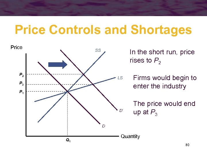
Price Controls and Shortages Price In the short run, price rises to P 2 SS P 2 LS P 3 P 1 D’ Firms would begin to enter the industry The price would end up at P 3 D Q 1 Quantity 80
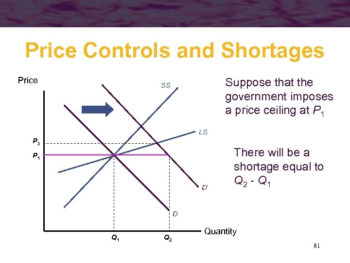
Price Controls and Shortages Price Suppose that the government imposes a price ceiling at P 1 SS LS P 3 P 1 D’ There will be a shortage equal to Q 2 - Q 1 D Q 1 Q 2 Quantity 81
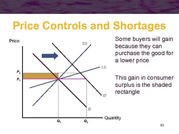
Price Controls and Shortages Price Some buyers will gain because they can purchase the good for a lower price SS LS P 3 P 1 D’ This gain in consumer surplus is the shaded rectangle D Q 1 Q 2 Quantity 82
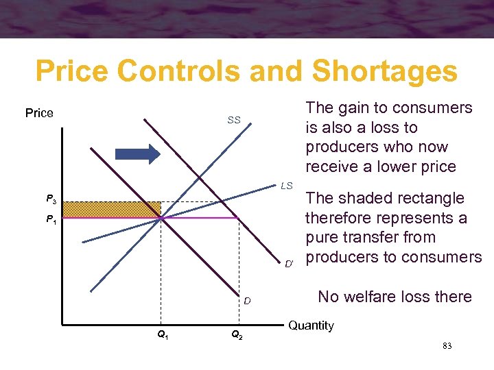
Price Controls and Shortages Price The gain to consumers is also a loss to producers who now receive a lower price SS LS P 3 P 1 D’ D Q 1 Q 2 The shaded rectangle therefore represents a pure transfer from producers to consumers No welfare loss there Quantity 83
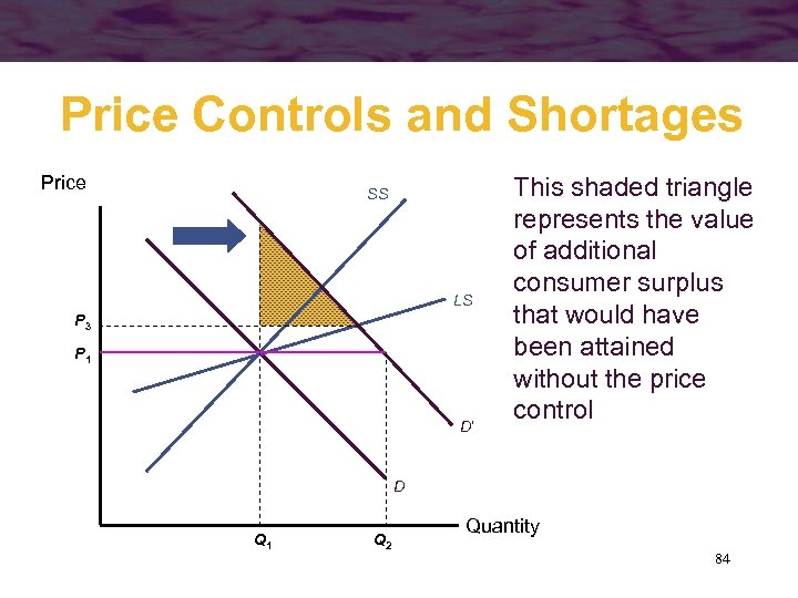
Price Controls and Shortages Price SS LS P 3 P 1 D’ This shaded triangle represents the value of additional consumer surplus that would have been attained without the price control D Q 1 Q 2 Quantity 84
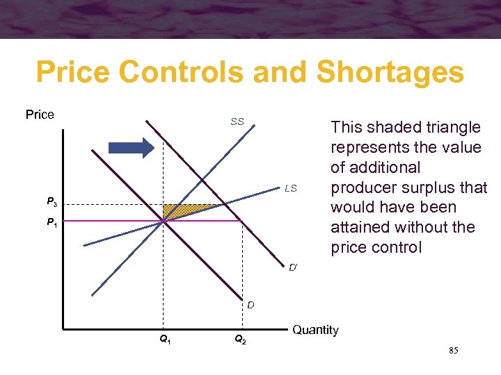
Price Controls and Shortages Price SS LS P 3 P 1 This shaded triangle represents the value of additional producer surplus that would have been attained without the price control D’ D Q 1 Q 2 Quantity 85
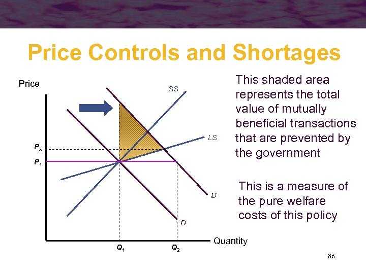
Price Controls and Shortages Price SS LS P 3 P 1 D’ D Q 1 Q 2 This shaded area represents the total value of mutually beneficial transactions that are prevented by the government This is a measure of the pure welfare costs of this policy Quantity 86

Disequilibrium Behavior • Notice that there are customers willing to pay more to buy the good • This could lead to a black market 87
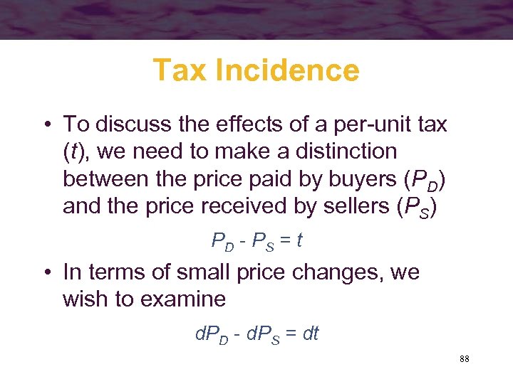
Tax Incidence • To discuss the effects of a per-unit tax (t), we need to make a distinction between the price paid by buyers (PD) and the price received by sellers (PS) PD - PS = t • In terms of small price changes, we wish to examine d. PD - d. PS = dt 88
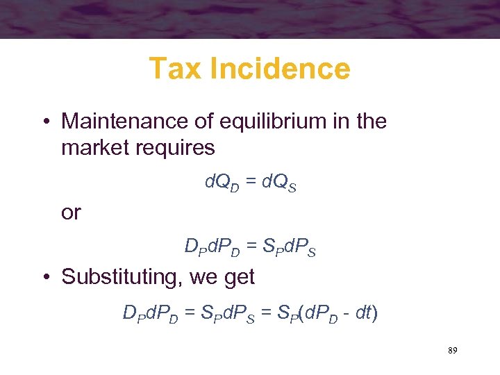
Tax Incidence • Maintenance of equilibrium in the market requires d. QD = d. QS or DPd. PD = SPd. PS • Substituting, we get DPd. PD = SPd. PS = SP(d. PD - dt) 89
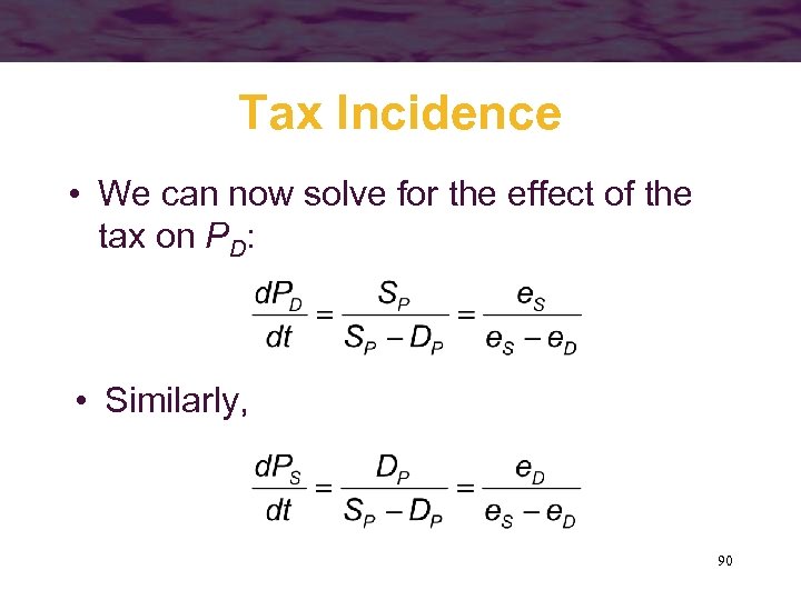
Tax Incidence • We can now solve for the effect of the tax on PD: • Similarly, 90
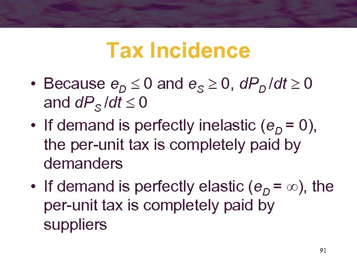
Tax Incidence • Because e. D 0 and e. S 0, d. PD /dt 0 and d. PS /dt 0 • If demand is perfectly inelastic (e. D = 0), the per-unit tax is completely paid by demanders • If demand is perfectly elastic (e. D = ), the per-unit tax is completely paid by suppliers 91
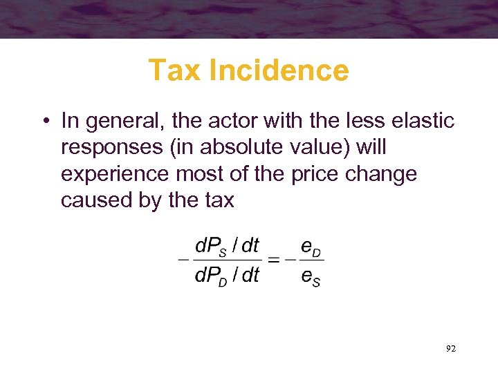
Tax Incidence • In general, the actor with the less elastic responses (in absolute value) will experience most of the price change caused by the tax 92
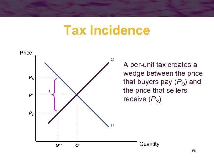
Tax Incidence Price S PD P* t A per-unit tax creates a wedge between the price that buyers pay (PD) and the price that sellers receive (PS) PS D Q** Q* Quantity 93
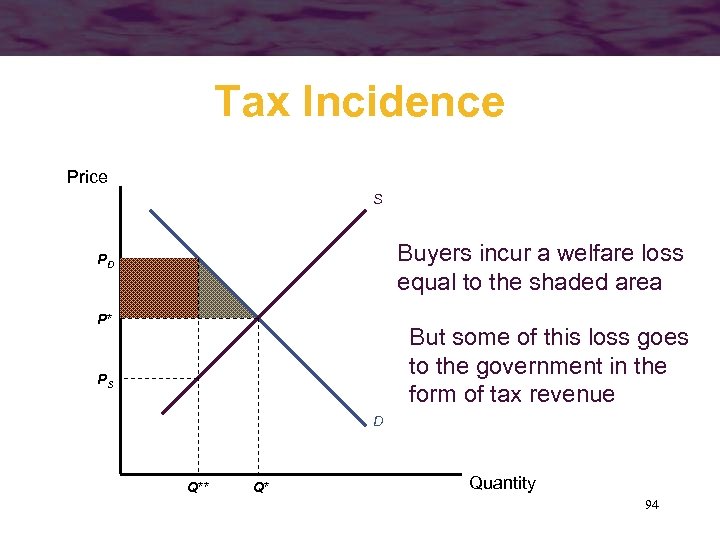
Tax Incidence Price S Buyers incur a welfare loss equal to the shaded area PD P* But some of this loss goes to the government in the form of tax revenue PS D Q** Q* Quantity 94
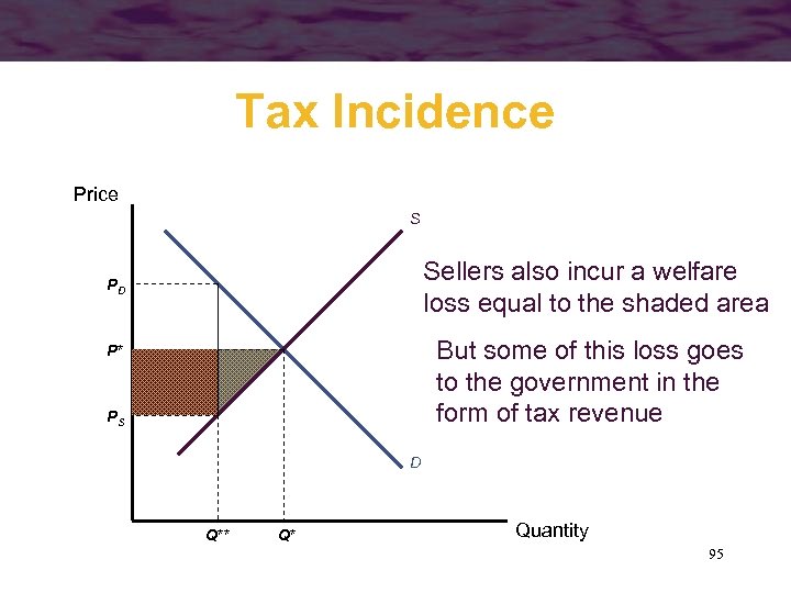
Tax Incidence Price S Sellers also incur a welfare loss equal to the shaded area PD But some of this loss goes to the government in the form of tax revenue P* PS D Q** Q* Quantity 95
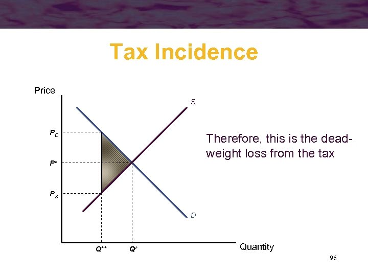
Tax Incidence Price S PD Therefore, this is the deadweight loss from the tax P* PS D Q** Q* Quantity 96
Deadweight Loss and Elasticity • All nonlump-sum taxes involve deadweight losses – the size of the losses will depend on the elasticities of supply and demand • A linear approximation to the deadweight loss accompanying a small tax, dt, is given by DW = -0. 5(dt)(d. Q) 97
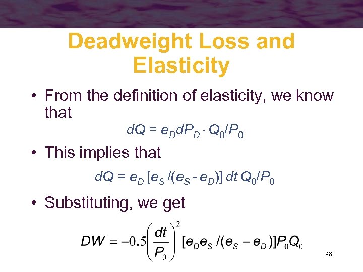
Deadweight Loss and Elasticity • From the definition of elasticity, we know that d. Q = e. Dd. PD Q 0/P 0 • This implies that d. Q = e. D [e. S /(e. S - e. D)] dt Q 0/P 0 • Substituting, we get 98
Deadweight Loss and Elasticity • Deadweight losses are zero if either e. D or e. S are zero – the tax does not alter the quantity of the good that is traded • Deadweight losses are smaller in situations where e. D or e. S are small 99
Transactions Costs • Transactions costs can also create a wedge between the price the buyer pays and the price the seller receives – real estate agent fees – broker fees for the sale of stocks • If the transactions costs are on a per-unit basis, these costs will be shared by the buyer and seller – depends on the specific elasticities involved 100
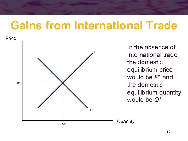
Gains from International Trade Price S P* In the absence of international trade, the domestic equilibrium price would be P* and the domestic equilibrium quantity would be Q* D Q* Quantity 101
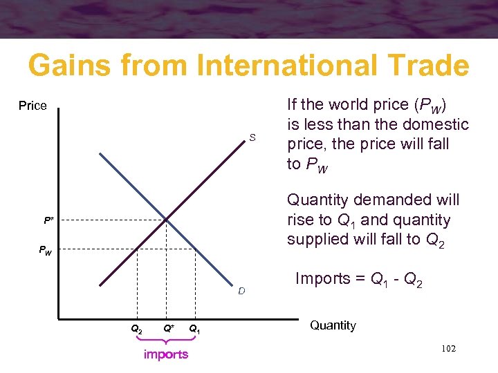
Gains from International Trade Price S If the world price (PW) is less than the domestic price, the price will fall to PW Quantity demanded will rise to Q 1 and quantity supplied will fall to Q 2 P* PW D Q 2 Q* Q 1 imports Imports = Q 1 - Q 2 Quantity 102
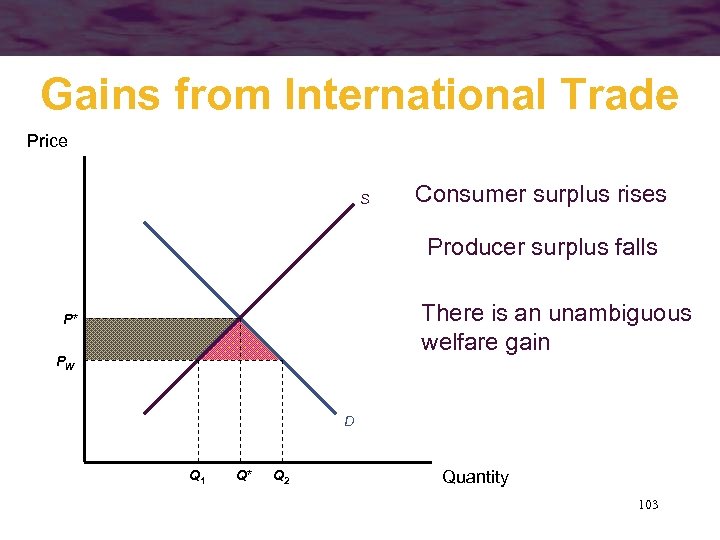
Gains from International Trade Price S Consumer surplus rises Producer surplus falls There is an unambiguous welfare gain P* PW D Q 1 Q* Q 2 Quantity 103
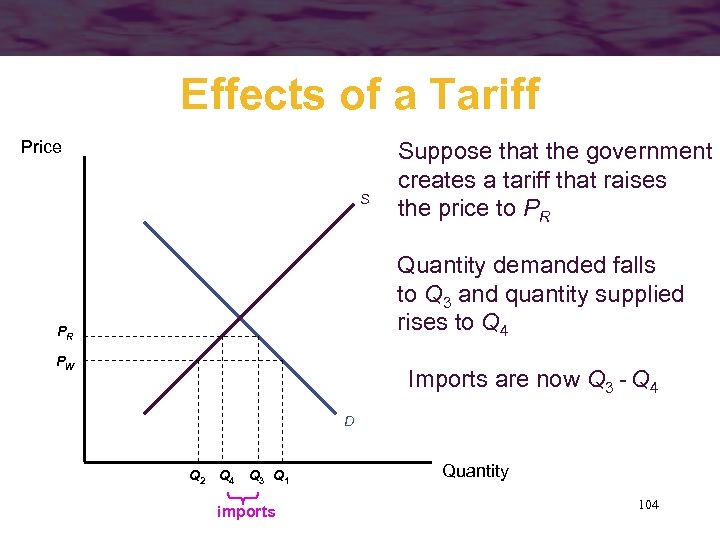
Effects of a Tariff Price S Suppose that the government creates a tariff that raises the price to PR Quantity demanded falls to Q 3 and quantity supplied rises to Q 4 PR PW Imports are now Q 3 - Q 4 D Q 2 Q 4 Q 3 Q 1 imports Quantity 104
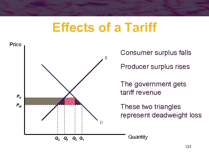
Effects of a Tariff Price S Consumer surplus falls Producer surplus rises The government gets tariff revenue PR These two triangles represent deadweight loss PW D Q 2 Q 4 Q 3 Q 1 Quantity 105
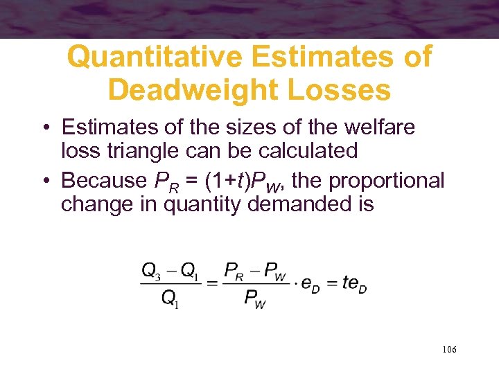
Quantitative Estimates of Deadweight Losses • Estimates of the sizes of the welfare loss triangle can be calculated • Because PR = (1+t)PW, the proportional change in quantity demanded is 106
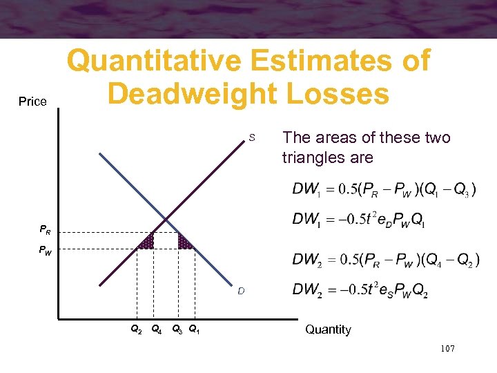
Price Quantitative Estimates of Deadweight Losses S The areas of these two triangles are PR PW D Q 2 Q 4 Q 3 Q 1 Quantity 107
Other Trade Restrictions • A quota that limits imports to Q 3 - Q 4 would have effects that are similar to those for the tariff – same decline in consumer surplus – same increase in producer surplus • One big difference is that the quota does not give the government any tariff revenue – the deadweight loss will be larger 108
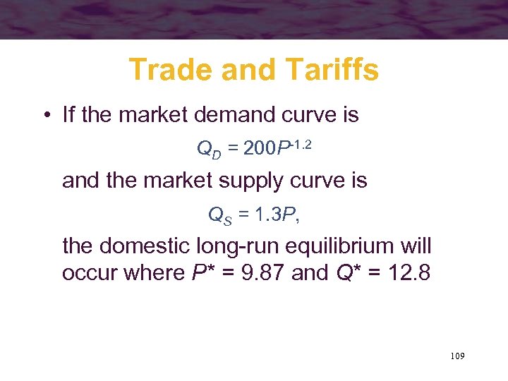
Trade and Tariffs • If the market demand curve is QD = 200 P-1. 2 and the market supply curve is QS = 1. 3 P, the domestic long-run equilibrium will occur where P* = 9. 87 and Q* = 12. 8 109
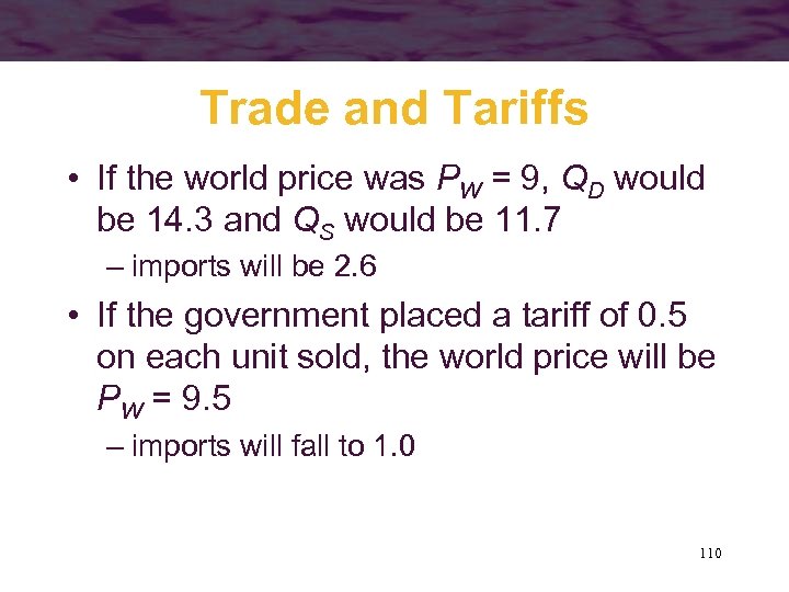
Trade and Tariffs • If the world price was PW = 9, QD would be 14. 3 and QS would be 11. 7 – imports will be 2. 6 • If the government placed a tariff of 0. 5 on each unit sold, the world price will be PW = 9. 5 – imports will fall to 1. 0 110
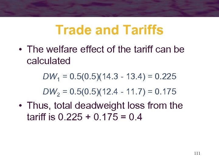
Trade and Tariffs • The welfare effect of the tariff can be calculated DW 1 = 0. 5(0. 5)(14. 3 - 13. 4) = 0. 225 DW 2 = 0. 5(0. 5)(12. 4 - 11. 7) = 0. 175 • Thus, total deadweight loss from the tariff is 0. 225 + 0. 175 = 0. 4 111
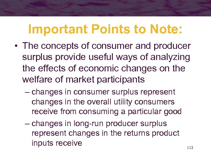
Important Points to Note: • The concepts of consumer and producer surplus provide useful ways of analyzing the effects of economic changes on the welfare of market participants – changes in consumer surplus represent changes in the overall utility consumers receive from consuming a particular good – changes in long-run producer surplus represent changes in the returns product inputs receive 112
Important Points to Note: • Price controls involve both transfers between producers and consumers and losses of transactions that could benefit both consumers and producers 113
Important Points to Note: • Tax incidence analysis concerns the determination of which economic actor ultimately bears the burden of a tax – this incidence will fall mainly on the actors who exhibit inelastic responses to price changes – taxes also involve deadweight losses that constitute an excess burden in addition to the burden imposed by the actual tax revenues collected 114
Important Points to Note: • Transaction costs can sometimes be modeled as taxes – both taxes and transaction costs may affect the attributes of transactions depending on the basis on which the costs are incurred 115
Important Points to Note: • Trade restrictions such as tariffs or quotas create transfers between consumers and producers and deadweight losses of economic welfare – the effects of many types of trade restrictions can be modeled as being equivalent to a per-unit tariff 116
bc1243ad3adc0c5ec990a4a21ce1bd94.ppt