9d9b06a1cec5d47a68c7f8f6361f990c.ppt
- Количество слайдов: 95
Chapter 10. Cluster Analysis: Basic Concepts and Methods n Cluster Analysis: Basic Concepts n Partitioning Methods n Hierarchical Methods n Density-Based Methods n Grid-Based Methods n Evaluation of Clustering 1
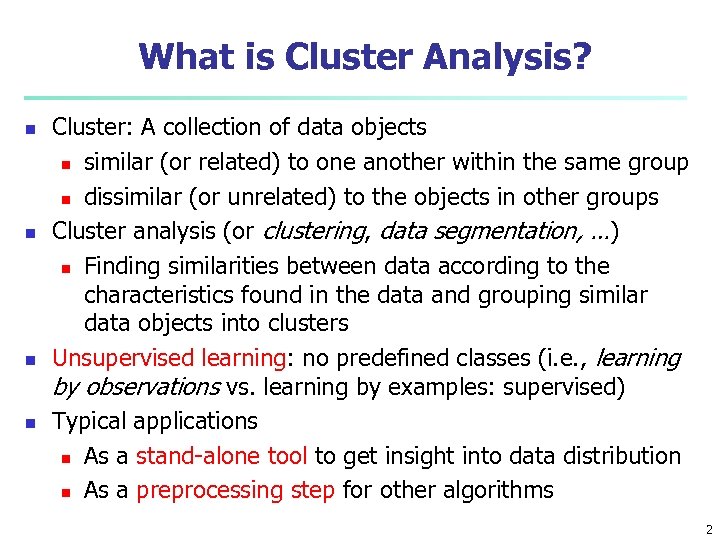
What is Cluster Analysis? n n Cluster: A collection of data objects n similar (or related) to one another within the same group n dissimilar (or unrelated) to the objects in other groups Cluster analysis (or clustering, data segmentation, …) n Finding similarities between data according to the characteristics found in the data and grouping similar data objects into clusters Unsupervised learning: no predefined classes (i. e. , learning by observations vs. learning by examples: supervised) Typical applications n As a stand-alone tool to get insight into data distribution n As a preprocessing step for other algorithms 2
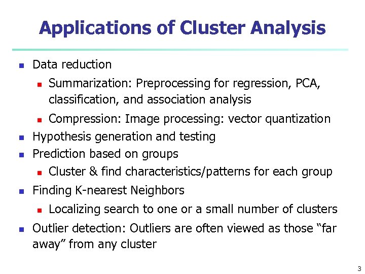
Applications of Cluster Analysis n Data reduction n Summarization: Preprocessing for regression, PCA, classification, and association analysis Compression: Image processing: vector quantization Hypothesis generation and testing Prediction based on groups n Cluster & find characteristics/patterns for each group n n Finding K-nearest Neighbors n n Localizing search to one or a small number of clusters Outlier detection: Outliers are often viewed as those “far away” from any cluster 3
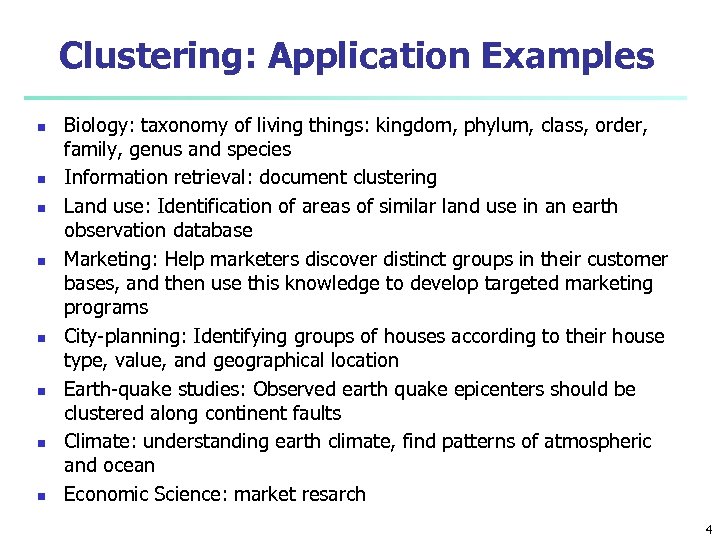
Clustering: Application Examples n n n n Biology: taxonomy of living things: kingdom, phylum, class, order, family, genus and species Information retrieval: document clustering Land use: Identification of areas of similar land use in an earth observation database Marketing: Help marketers discover distinct groups in their customer bases, and then use this knowledge to develop targeted marketing programs City-planning: Identifying groups of houses according to their house type, value, and geographical location Earth-quake studies: Observed earth quake epicenters should be clustered along continent faults Climate: understanding earth climate, find patterns of atmospheric and ocean Economic Science: market resarch 4
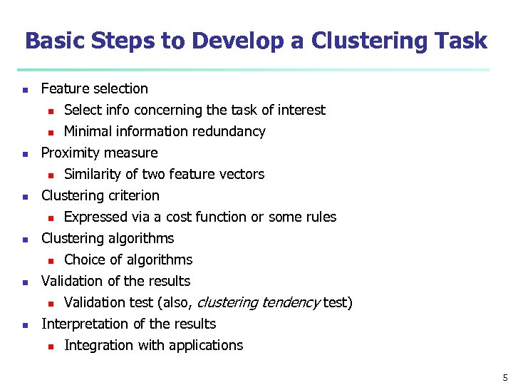
Basic Steps to Develop a Clustering Task n Feature selection n Select info concerning the task of interest Minimal information redundancy Proximity measure n Similarity of two feature vectors Clustering criterion n Expressed via a cost function or some rules Clustering algorithms n Choice of algorithms Validation of the results n Validation test (also, clustering tendency test) Interpretation of the results n Integration with applications n n n 5
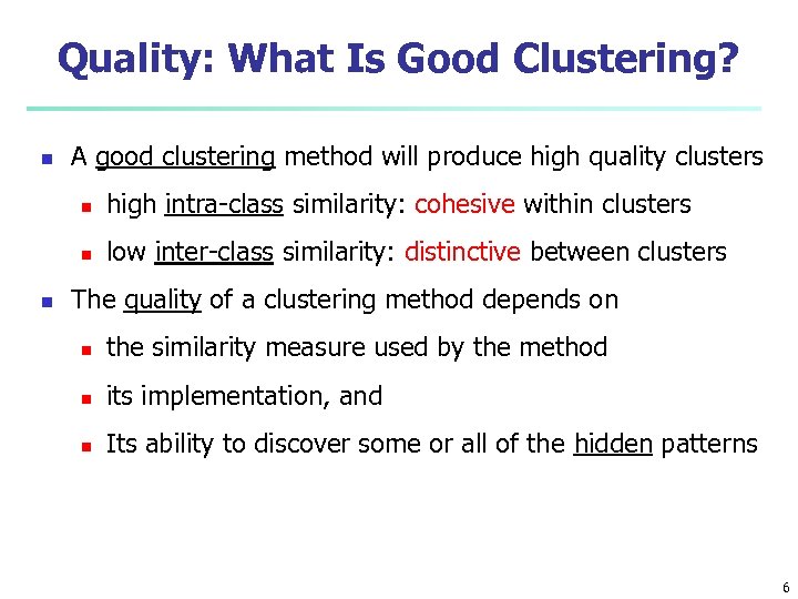
Quality: What Is Good Clustering? n A good clustering method will produce high quality clusters n n n high intra-class similarity: cohesive within clusters low inter-class similarity: distinctive between clusters The quality of a clustering method depends on n the similarity measure used by the method n its implementation, and n Its ability to discover some or all of the hidden patterns 6
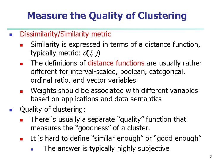
Measure the Quality of Clustering n n Dissimilarity/Similarity metric n Similarity is expressed in terms of a distance function, typically metric: d(i, j) n The definitions of distance functions are usually rather different for interval-scaled, boolean, categorical, ordinal ratio, and vector variables n Weights should be associated with different variables based on applications and data semantics Quality of clustering: n There is usually a separate “quality” function that measures the “goodness” of a cluster. n It is hard to define “similar enough” or “good enough” n The answer is typically highly subjective 7
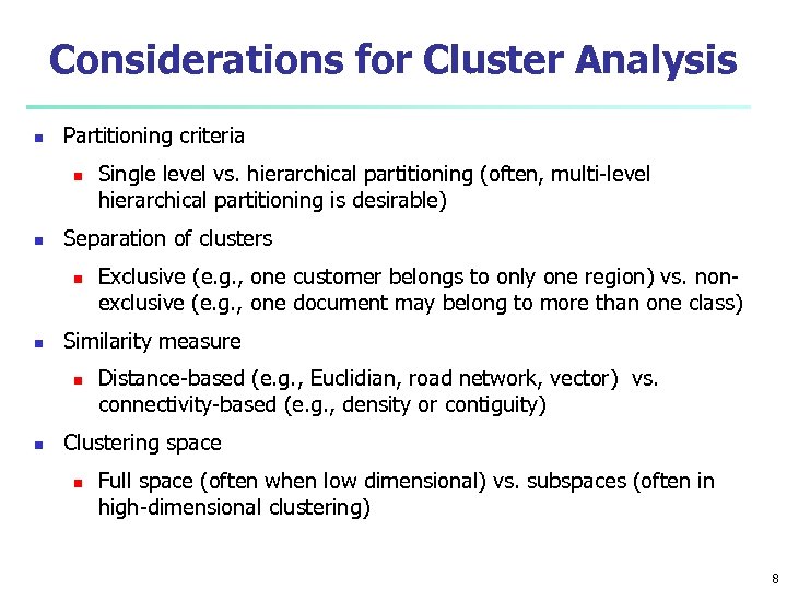
Considerations for Cluster Analysis n Partitioning criteria n n Separation of clusters n n Exclusive (e. g. , one customer belongs to only one region) vs. nonexclusive (e. g. , one document may belong to more than one class) Similarity measure n n Single level vs. hierarchical partitioning (often, multi-level hierarchical partitioning is desirable) Distance-based (e. g. , Euclidian, road network, vector) vs. connectivity-based (e. g. , density or contiguity) Clustering space n Full space (often when low dimensional) vs. subspaces (often in high-dimensional clustering) 8
Requirements and Challenges n n n Scalability n Clustering all the data instead of only on samples Ability to deal with different types of attributes n Numerical, binary, categorical, ordinal, linked, and mixture of these Constraint-based clustering n User may give inputs on constraints n Use domain knowledge to determine input parameters Interpretability and usability Others n Discovery of clusters with arbitrary shape n Ability to deal with noisy data n Incremental clustering and insensitivity to input order n High dimensionality 9
Major Clustering Approaches (I) n n Partitioning approach: n Construct various partitions and then evaluate them by some criterion, e. g. , minimizing the sum of square errors n Typical methods: k-means, k-medoids, CLARANS Hierarchical approach: n Create a hierarchical decomposition of the set of data (or objects) using some criterion n Typical methods: Diana, Agnes, BIRCH, CAMELEON Density-based approach: n Based on connectivity and density functions n Typical methods: DBSACN, OPTICS, Den. Clue Grid-based approach: n based on a multiple-level granularity structure n Typical methods: STING, Wave. Cluster, CLIQUE 10
Major Clustering Approaches (II) n n Model-based: n A model is hypothesized for each of the clusters and tries to find the best fit of that model to each other n Typical methods: EM, SOM, COBWEB Frequent pattern-based: n Based on the analysis of frequent patterns n Typical methods: p-Cluster User-guided or constraint-based: n Clustering by considering user-specified or application-specific constraints n Typical methods: COD (obstacles), constrained clustering Link-based clustering: n Objects are often linked together in various ways n Massive links can be used to cluster objects: Sim. Rank, Link. Clus 11
Chapter 10. Cluster Analysis: Basic Concepts and Methods n Cluster Analysis: Basic Concepts n Partitioning Methods n Hierarchical Methods n Density-Based Methods n Grid-Based Methods n Evaluation of Clustering 12
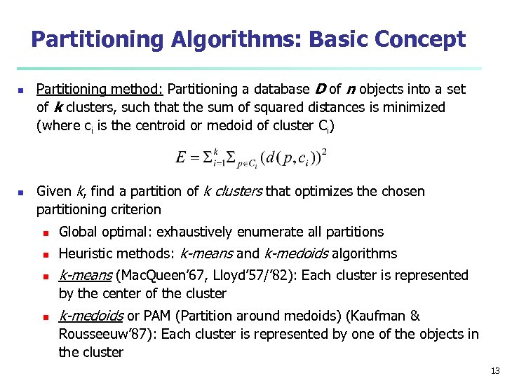
Partitioning Algorithms: Basic Concept n n Partitioning method: Partitioning a database D of n objects into a set of k clusters, such that the sum of squared distances is minimized (where ci is the centroid or medoid of cluster Ci) Given k, find a partition of k clusters that optimizes the chosen partitioning criterion n Global optimal: exhaustively enumerate all partitions n Heuristic methods: k-means and k-medoids algorithms n k-means (Mac. Queen’ 67, Lloyd’ 57/’ 82): Each cluster is represented by the center of the cluster n k-medoids or PAM (Partition around medoids) (Kaufman & Rousseeuw’ 87): Each cluster is represented by one of the objects in the cluster 13
The K-Means Clustering Method n Given k, the k-means algorithm is implemented in four steps: n n Partition objects into k nonempty subsets Compute seed points as the centroids of the clusters of the current partitioning (the centroid is the center, i. e. , mean point, of the cluster) Assign each object to the cluster with the nearest seed point Go back to Step 2, stop when the assignment does not change 14
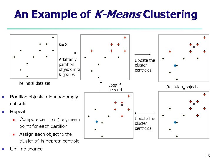
An Example of K-Means Clustering K=2 Arbitrarily partition objects into k groups The initial data set n n Loop if needed Reassign objects Partition objects into k nonempty subsets Repeat n n n Update the cluster centroids Compute centroid (i. e. , mean point) for each partition Update the cluster centroids Assign each object to the cluster of its nearest centroid Until no change 15
Comments on the K-Means Method n Strength: Efficient: O(tkn), where n is # objects, k is # clusters, and t is # iterations. Normally, k, t << n. n Comparing: PAM: O(k(n-k)2 ), CLARA: O(ks 2 + k(n-k)) n Comment: Often terminates at a local optimal n Weakness n Applicable only to objects in a continuous n-dimensional space n n n Using the k-modes method for categorical data In comparison, k-medoids can be applied to a wide range of data Need to specify k, the number of clusters, in advance (there are ways to automatically determine the best k (see Hastie et al. , 2009) n Sensitive to noisy data and outliers n Not suitable to discover clusters with non-convex shapes 16
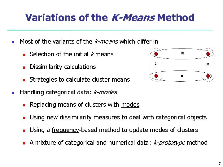
Variations of the K-Means Method n Most of the variants of the k-means which differ in n n Dissimilarity calculations n n Selection of the initial k means Strategies to calculate cluster means Handling categorical data: k-modes n Replacing means of clusters with modes n Using new dissimilarity measures to deal with categorical objects n Using a frequency-based method to update modes of clusters n A mixture of categorical and numerical data: k-prototype method 17
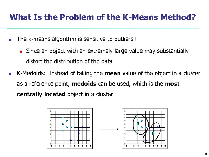
What Is the Problem of the K-Means Method? n The k-means algorithm is sensitive to outliers ! n Since an object with an extremely large value may substantially distort the distribution of the data n K-Medoids: Instead of taking the mean value of the object in a cluster as a reference point, medoids can be used, which is the most centrally located object in a cluster 10 10 9 9 8 8 7 7 6 6 5 5 4 4 3 3 2 2 1 1 0 0 0 1 2 3 4 5 6 7 8 9 10 18
The K-Medoid Clustering Method n K-Medoids Clustering: Find representative objects (medoids) in clusters n PAM (Partitioning Around Medoids, Kaufmann & Rousseeuw 1987) n Starts from an initial set of medoids and iteratively replaces one of the medoids by one of the non-medoids if it improves the total distance of the resulting clustering n PAM works effectively for small data sets, but does not scale well for large data sets (due to the computational complexity) n Efficiency improvement on PAM n CLARA (Kaufmann & Rousseeuw, 1990): PAM on samples n CLARANS (Ng & Han, 1994): Randomized re-sampling 19
Chapter 10. Cluster Analysis: Basic Concepts and Methods n Cluster Analysis: Basic Concepts n Partitioning Methods n Hierarchical Methods n Density-Based Methods n Grid-Based Methods n Evaluation of Clustering 20
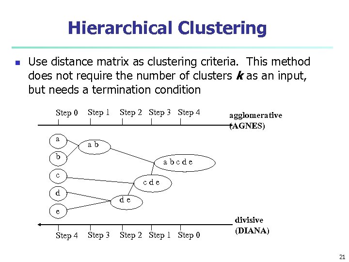
Hierarchical Clustering n Use distance matrix as clustering criteria. This method does not require the number of clusters k as an input, but needs a termination condition Step 0 a Step 1 Step 2 Step 3 Step 4 ab b abcde c cde d de e Step 4 agglomerative (AGNES) Step 3 Step 2 Step 1 Step 0 divisive (DIANA) 21
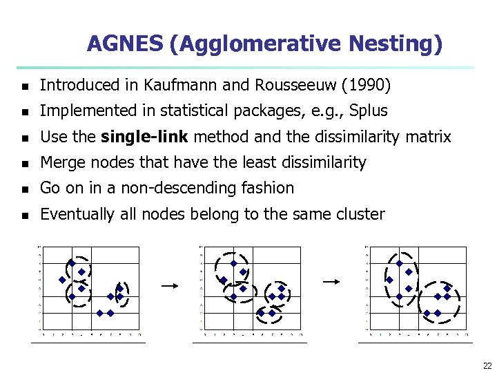
AGNES (Agglomerative Nesting) n Introduced in Kaufmann and Rousseeuw (1990) n Implemented in statistical packages, e. g. , Splus n Use the single-link method and the dissimilarity matrix n Merge nodes that have the least dissimilarity n Go on in a non-descending fashion n Eventually all nodes belong to the same cluster 22
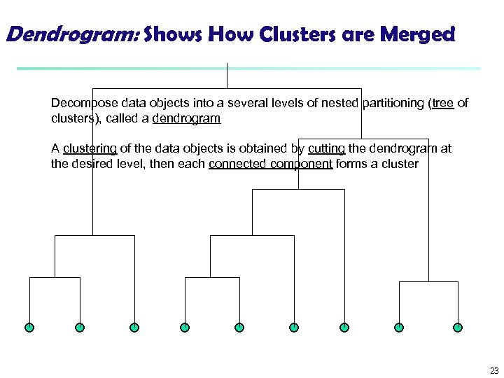
Dendrogram: Shows How Clusters are Merged Decompose data objects into a several levels of nested partitioning (tree of clusters), called a dendrogram A clustering of the data objects is obtained by cutting the dendrogram at the desired level, then each connected component forms a cluster 23
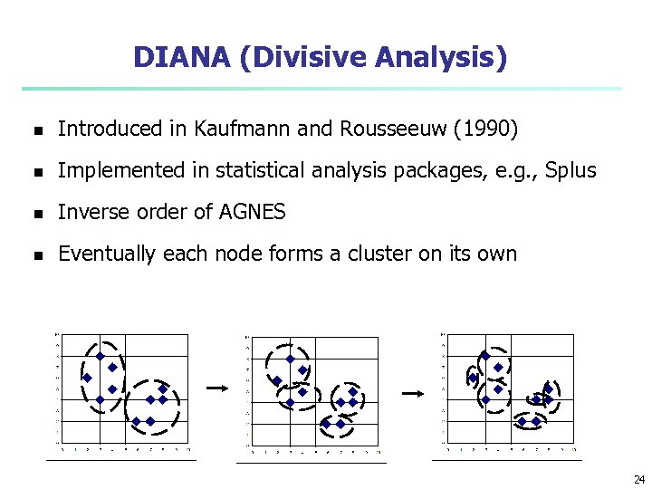
DIANA (Divisive Analysis) n Introduced in Kaufmann and Rousseeuw (1990) n Implemented in statistical analysis packages, e. g. , Splus n Inverse order of AGNES n Eventually each node forms a cluster on its own 24
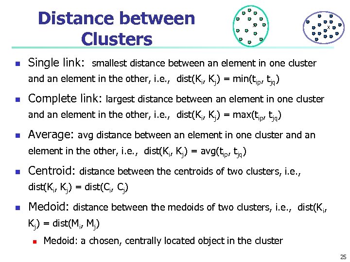
Distance between Clusters n X X Single link: smallest distance between an element in one cluster and an element in the other, i. e. , dist(Ki, Kj) = min(tip, tjq) n Complete link: largest distance between an element in one cluster and an element in the other, i. e. , dist(Ki, Kj) = max(tip, tjq) n Average: avg distance between an element in one cluster and an element in the other, i. e. , dist(Ki, Kj) = avg(tip, tjq) n Centroid: distance between the centroids of two clusters, i. e. , dist(Ki, Kj) = dist(Ci, Cj) n Medoid: distance between the medoids of two clusters, i. e. , dist(Ki, Kj) = dist(Mi, Mj) n Medoid: a chosen, centrally located object in the cluster 25
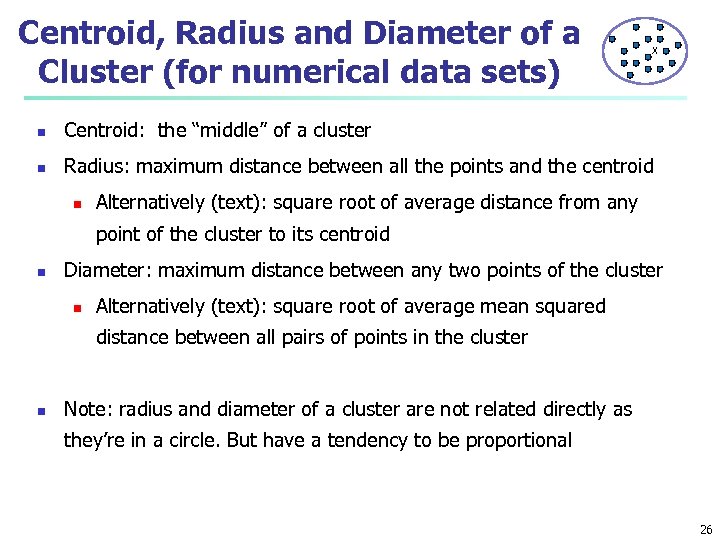
Centroid, Radius and Diameter of a Cluster (for numerical data sets) X n Centroid: the “middle” of a cluster n Radius: maximum distance between all the points and the centroid n Alternatively (text): square root of average distance from any point of the cluster to its centroid n Diameter: maximum distance between any two points of the cluster n Alternatively (text): square root of average mean squared distance between all pairs of points in the cluster n Note: radius and diameter of a cluster are not related directly as they’re in a circle. But have a tendency to be proportional 26
Extensions to Hierarchical Clustering n Major weakness of agglomerative clustering methods n Can never undo what was done previously n Do not scale well: time complexity of at least O(n 2), where n is the number of total objects n Integration of hierarchical & distance-based clustering n BIRCH (1996): uses CF-tree and incrementally adjusts the quality of sub-clusters n CHAMELEON (1999): hierarchical clustering using dynamic modeling 27
BIRCH (Balanced Iterative Reducing and Clustering Using Hierarchies) n n Zhang, Ramakrishnan & Livny, SIGMOD’ 96 Incrementally construct a CF (Clustering Feature) tree, a hierarchical data structure for multiphase clustering n n n Phase 1: scan DB to build an initial in-memory CF tree (a multi-level compression of the data that tries to preserve the inherent clustering structure of the data) Phase 2: use an arbitrary clustering algorithm to cluster the leaf nodes of the CF-tree Scales linearly: finds a good clustering with a single scan and improves the quality with a few additional scans n Weakness: handles only numeric data, and sensitive to the order of the data record 28
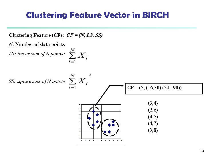
Clustering Feature Vector in BIRCH Clustering Feature (CF): CF = (N, LS, SS) N: Number of data points LS: linear sum of N points: SS: square sum of N points CF = (5, (16, 30), (54, 190)) (3, 4) (2, 6) (4, 5) (4, 7) (3, 8) 29
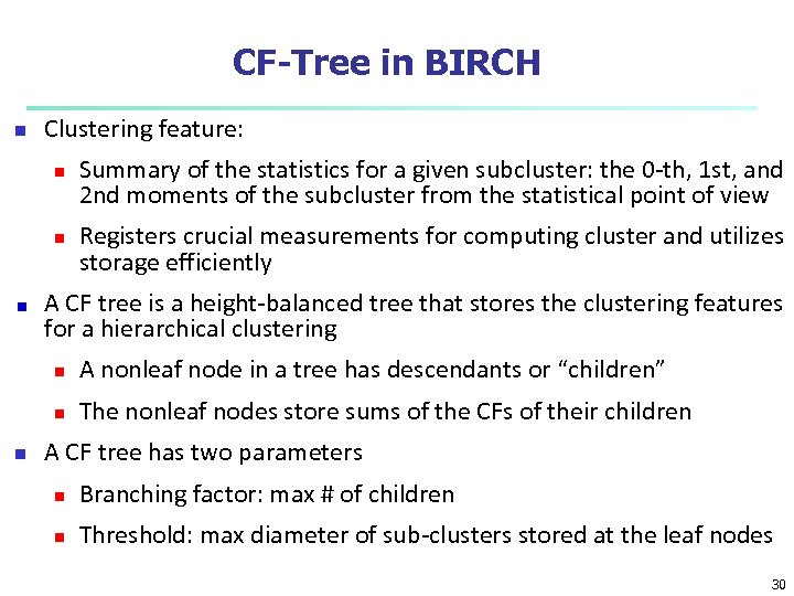
CF-Tree in BIRCH n Clustering feature: n n Summary of the statistics for a given subcluster: the 0 -th, 1 st, and 2 nd moments of the subcluster from the statistical point of view Registers crucial measurements for computing cluster and utilizes storage efficiently A CF tree is a height-balanced tree that stores the clustering features for a hierarchical clustering n n n A nonleaf node in a tree has descendants or “children” The nonleaf nodes store sums of the CFs of their children A CF tree has two parameters n Branching factor: max # of children n Threshold: max diameter of sub-clusters stored at the leaf nodes 30
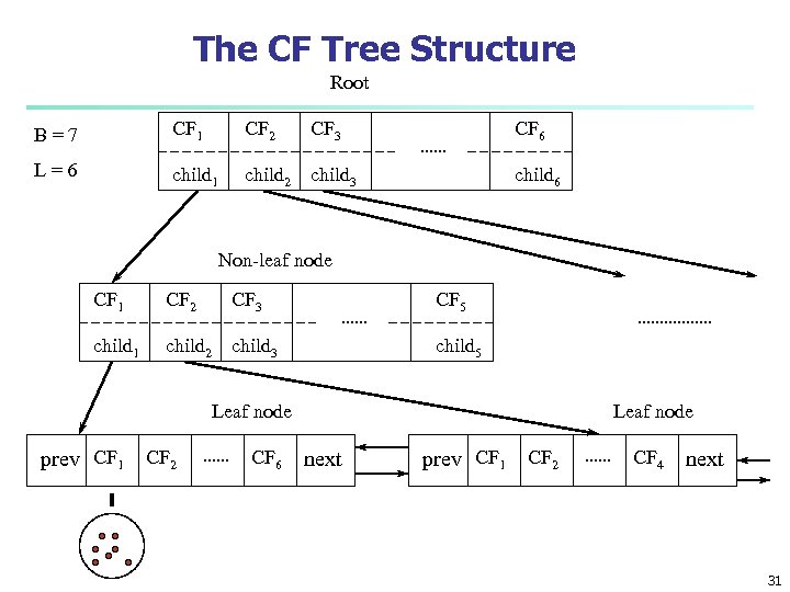
The CF Tree Structure Root B=7 CF 1 CF 2 CF 3 CF 6 L=6 child 1 child 2 child 3 child 6 Non-leaf node CF 1 CF 2 CF 3 CF 5 child 1 child 2 child 3 child 5 Leaf node prev CF 1 CF 2 CF 6 Leaf node next prev CF 1 CF 2 CF 4 next 31
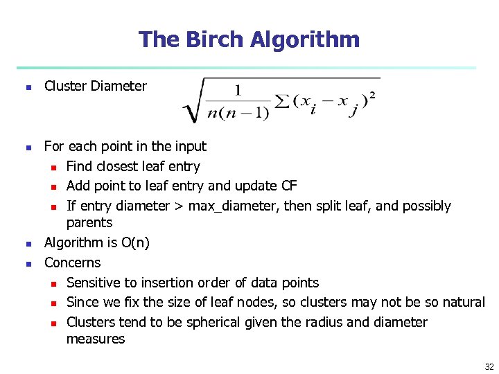
The Birch Algorithm n n Cluster Diameter For each point in the input n Find closest leaf entry n Add point to leaf entry and update CF n If entry diameter > max_diameter, then split leaf, and possibly parents Algorithm is O(n) Concerns n Sensitive to insertion order of data points n Since we fix the size of leaf nodes, so clusters may not be so natural n Clusters tend to be spherical given the radius and diameter measures 32
CHAMELEON: Hierarchical Clustering Using Dynamic Modeling (1999) n CHAMELEON: G. Karypis, E. H. Han, and V. Kumar, 1999 n Measures the similarity based on a dynamic model n n Two clusters are merged only if the interconnectivity and closeness (proximity) between two clusters are high relative to the internal interconnectivity of the clusters and closeness of items within the clusters Graph-based, and a two-phase algorithm 1. 2. Use a graph-partitioning algorithm: cluster objects into a large number of relatively small sub-clusters Use an agglomerative hierarchical clustering algorithm: find the genuine clusters by repeatedly combining these sub-clusters 33
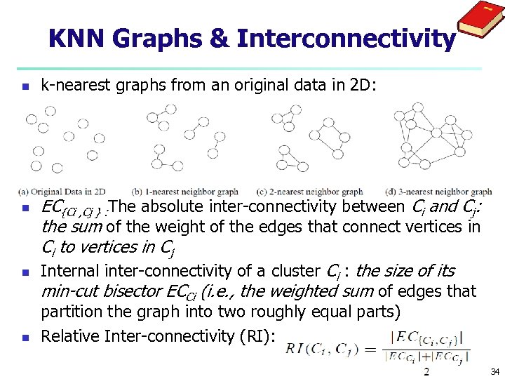
KNN Graphs & Interconnectivity n n k-nearest graphs from an original data in 2 D: EC{Ci , Cj } : The absolute inter-connectivity between Ci and Cj: the sum of the weight of the edges that connect vertices in Ci to vertices in Cj Internal inter-connectivity of a cluster Ci : the size of its min-cut bisector ECCi (i. e. , the weighted sum of edges that partition the graph into two roughly equal parts) Relative Inter-connectivity (RI): 34
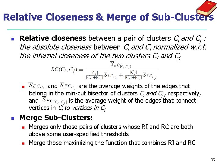
Relative Closeness & Merge of Sub-Clusters n Relative closeness between a pair of clusters Ci and Cj : the absolute closeness between Ci and Cj normalized w. r. t. the internal closeness of the two clusters Ci and Cj n n and are the average weights of the edges that belong in the min-cut bisector of clusters Ci and Cj , respectively, and is the average weight of the edges that connect vertices in Ci to vertices in Cj Merge Sub-Clusters: n n Merges only those pairs of clusters whose RI and RC are both above some user-specified thresholds Merge those maximizing the function that combines RI and RC 35
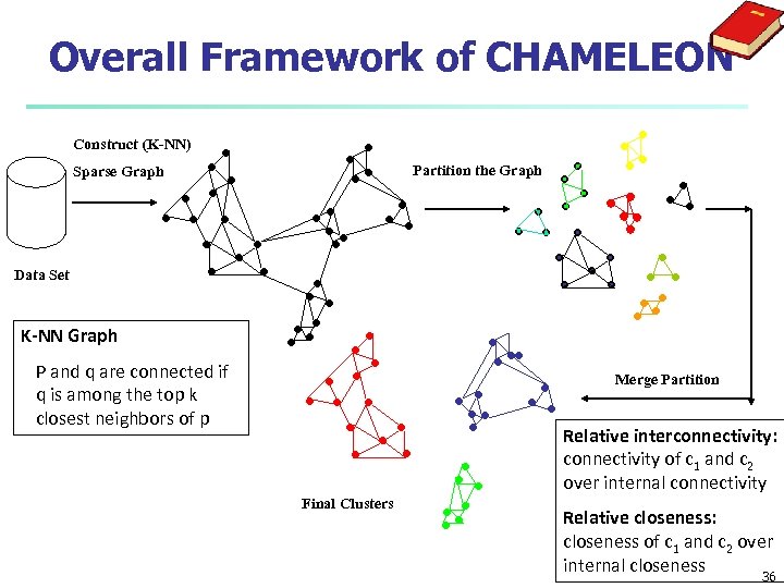
Overall Framework of CHAMELEON Construct (K-NN) Partition the Graph Sparse Graph Data Set K-NN Graph P and q are connected if q is among the top k closest neighbors of p Merge Partition Relative interconnectivity: connectivity of c 1 and c 2 over internal connectivity Final Clusters Relative closeness: closeness of c 1 and c 2 over internal closeness 36
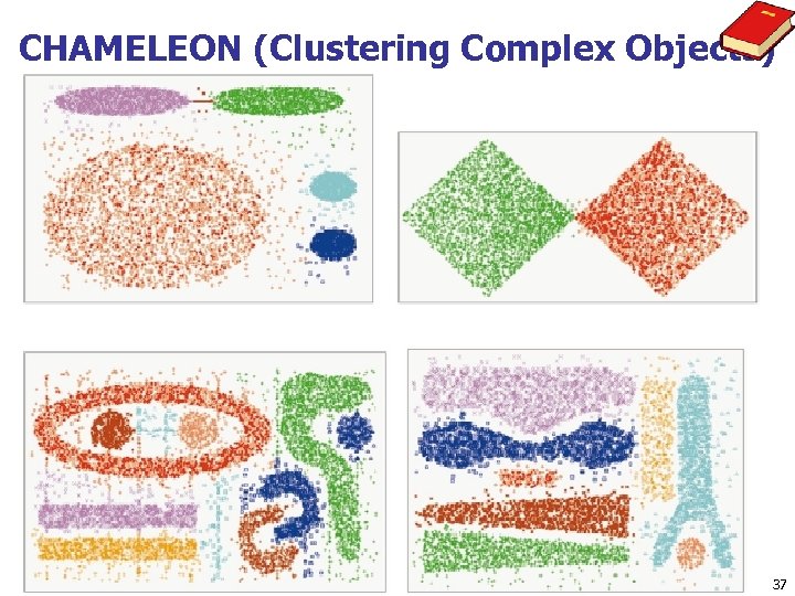
CHAMELEON (Clustering Complex Objects) 37
Chapter 10. Cluster Analysis: Basic Concepts and Methods n Cluster Analysis: Basic Concepts n Partitioning Methods n Hierarchical Methods n Density-Based Methods n Grid-Based Methods n Evaluation of Clustering 38
Density-Based Clustering Methods n n n Clustering based on density (local cluster criterion), such as density-connected points Major features: n Discover clusters of arbitrary shape n Handle noise n One scan n Need density parameters as termination condition Several interesting studies: n DBSCAN: Ester, et al. (KDD’ 96) n OPTICS: Ankerst, et al (SIGMOD’ 99). n DENCLUE: Hinneburg & D. Keim (KDD’ 98) n CLIQUE: Agrawal, et al. (SIGMOD’ 98) (more grid-based) 39
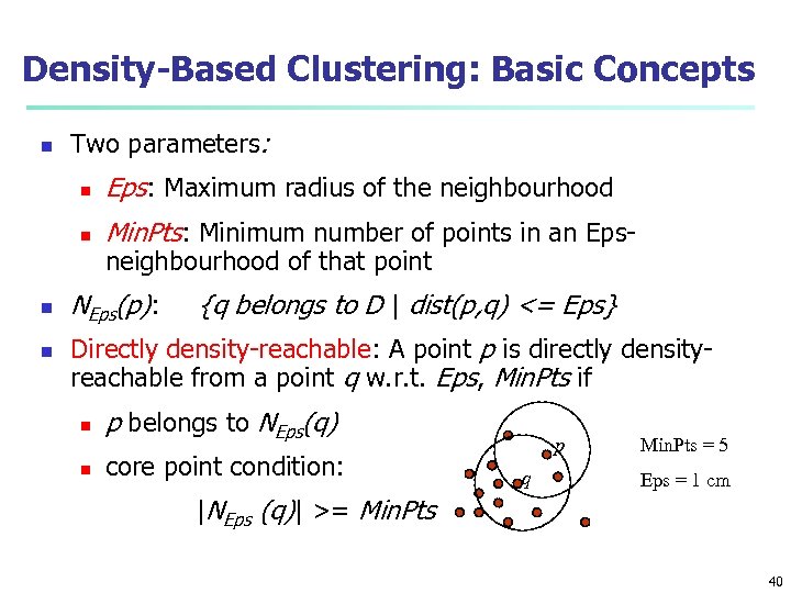
Density-Based Clustering: Basic Concepts n Two parameters: n n Eps: Maximum radius of the neighbourhood Min. Pts: Minimum number of points in an Epsneighbourhood of that point NEps(p): {q belongs to D | dist(p, q) <= Eps} Directly density-reachable: A point p is directly densityreachable from a point q w. r. t. Eps, Min. Pts if n p belongs to NEps(q) n core point condition: p q Min. Pts = 5 Eps = 1 cm |NEps (q)| >= Min. Pts 40
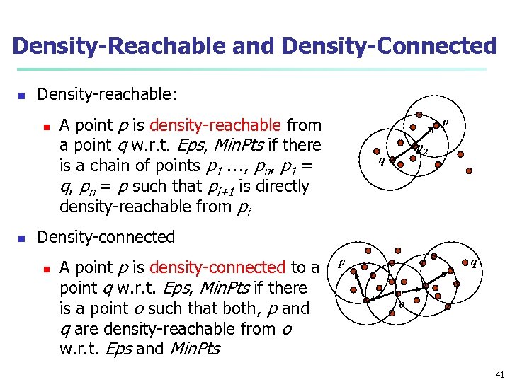
Density-Reachable and Density-Connected n Density-reachable: n n A point p is density-reachable from a point q w. r. t. Eps, Min. Pts if there is a chain of points p 1 …, pn, p 1 = q, pn = p such that pi+1 is directly density-reachable from pi p p 2 q Density-connected n A point p is density-connected to a point q w. r. t. Eps, Min. Pts if there is a point o such that both, p and q are density-reachable from o w. r. t. Eps and Min. Pts p q o 41
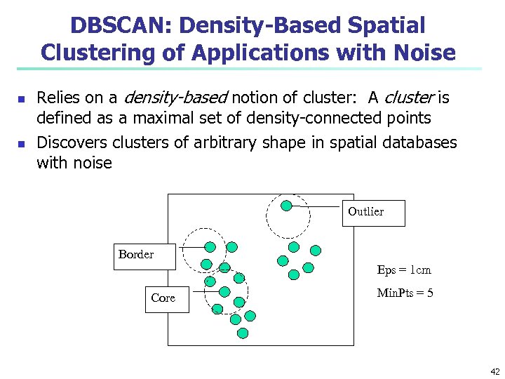
DBSCAN: Density-Based Spatial Clustering of Applications with Noise n n Relies on a density-based notion of cluster: A cluster is defined as a maximal set of density-connected points Discovers clusters of arbitrary shape in spatial databases with noise Outlier Border Eps = 1 cm Core Min. Pts = 5 42
DBSCAN: The Algorithm n n n Arbitrary select a point p Retrieve all points density-reachable from p w. r. t. Eps and Min. Pts If p is a core point, a cluster is formed If p is a border point, no points are density-reachable from p and DBSCAN visits the next point of the database Continue the process until all of the points have been processed If a spatial index is used, the computational complexity of DBSCAN is O(nlogn), where n is the number of database objects. Otherwise, the complexity is O(n 2) 43
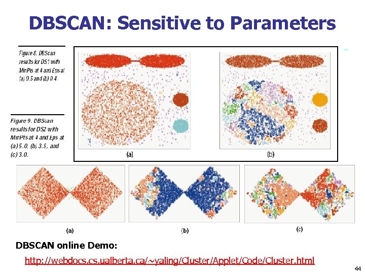
DBSCAN: Sensitive to Parameters DBSCAN online Demo: http: //webdocs. ualberta. ca/~yaling/Cluster/Applet/Code/Cluster. html 44
OPTICS: A Cluster-Ordering Method (1999) n OPTICS: Ordering Points To Identify the Clustering Structure n Ankerst, Breunig, Kriegel, and Sander (SIGMOD’ 99) n Produces a special order of the database wrt its density -based clustering structure n This cluster-ordering contains info equiv to the densitybased clusterings corresponding to a broad range of parameter settings n Good for both automatic and interactive cluster analysis, including finding intrinsic clustering structure n Can be represented graphically or using visualization techniques 45
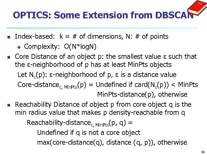
OPTICS: Some Extension from DBSCAN n n n Index-based: k = # of dimensions, N: # of points n Complexity: O(N*log. N) Core Distance of an object p: the smallest value ε such that the ε-neighborhood of p has at least Min. Pts objects Let Nε(p): ε-neighborhood of p, ε is a distance value Core-distanceε, Min. Pts(p) = Undefined if card(Nε(p)) < Min. Pts-distance(p), otherwise Reachability Distance of object p from core object q is the min radius value that makes p density-reachable from q Reachability-distanceε, Min. Pts(p, q) = Undefined if q is not a core object max(core-distance(q), distance (q, p)), otherwise 46
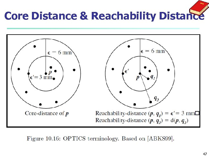
Core Distance & Reachability Distance 47
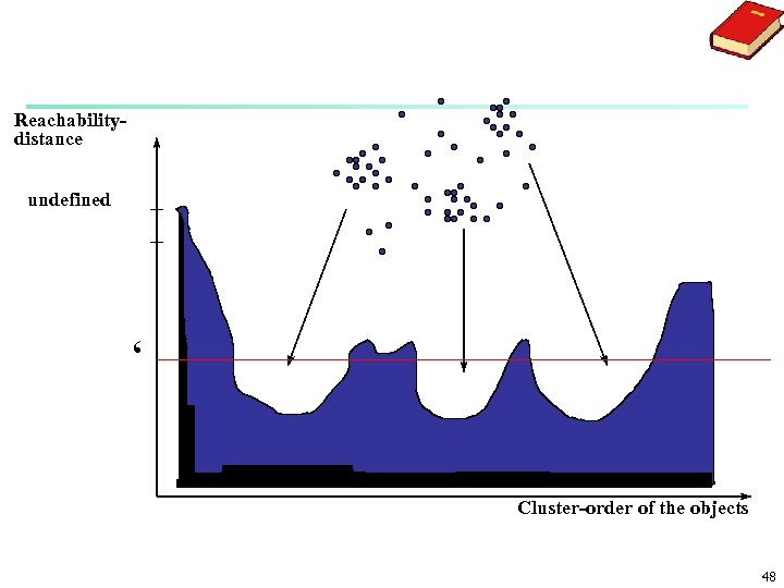
Reachabilitydistance undefined ‘ Cluster-order of the objects 48
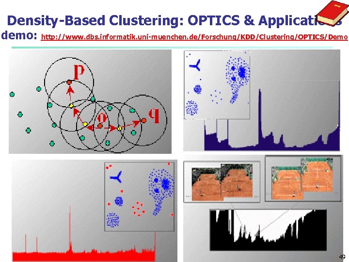
Density-Based Clustering: OPTICS & Applications demo: http: //www. dbs. informatik. uni-muenchen. de/Forschung/KDD/Clustering/OPTICS/Demo 49
Chapter 10. Cluster Analysis: Basic Concepts and Methods n Cluster Analysis: Basic Concepts n Partitioning Methods n Hierarchical Methods n Density-Based Methods n Grid-Based Methods n Evaluation of Clustering 50
Grid-Based Clustering Method n n Using multi-resolution grid data structure Several interesting methods n STING (a STatistical INformation Grid approach) by Wang, Yang and Muntz (1997) n CLIQUE: Agrawal, et al. (SIGMOD’ 98) n n Both grid-based and subspace clustering Wave. Cluster by Sheikholeslami, Chatterjee, and Zhang (VLDB’ 98) n A multi-resolution clustering approach using wavelet method 51
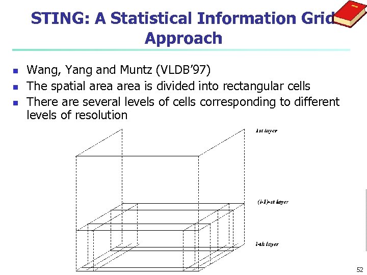
STING: A Statistical Information Grid Approach n n n Wang, Yang and Muntz (VLDB’ 97) The spatial area is divided into rectangular cells There are several levels of cells corresponding to different levels of resolution 52
The STING Clustering Method n n n Each cell at a high level is partitioned into a number of smaller cells in the next lower level Statistical info of each cell is calculated and stored beforehand is used to answer queries Parameters of higher level cells can be easily calculated from parameters of lower level cell n count, mean, s, min, max n type of distribution—normal, uniform, etc. Use a top-down approach to answer spatial data queries Start from a pre-selected layer—typically with a small number of cells For each cell in the current level compute the confidence interval 53
STING Algorithm and Its Analysis n n n Remove the irrelevant cells from further consideration When finish examining the current layer, proceed to the next lower level Repeat this process until the bottom layer is reached Advantages: n Query-independent, easy to parallelize, incremental update n O(K), where K is the number of grid cells at the lowest level Disadvantages: n All the cluster boundaries are either horizontal or vertical, and no diagonal boundary is detected 54
Chapter 10. Cluster Analysis: Basic Concepts and Methods n Cluster Analysis: Basic Concepts n Partitioning Methods n Hierarchical Methods n Density-Based Methods n Grid-Based Methods n Evaluation of Clustering 55
Measuring Clustering Quality n 3 kinds of measures: External, internal and relative n External: supervised, employ criteria not inherent to the dataset n n Internal: unsupervised, criteria derived from data itself n n Compare a clustering against prior or expert-specified knowledge (i. e. , the ground truth) using certain clustering quality measure Evaluate the goodness of a clustering by considering how well the clusters are separated, and how compact the clusters are, e. g. , Silhouette coefficient Relative: directly compare different clusterings, usually those obtained via different parameter settings for the same algorithm 56
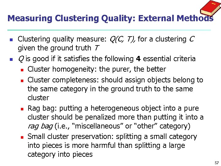
Measuring Clustering Quality: External Methods n n Clustering quality measure: Q(C, T), for a clustering C given the ground truth T Q is good if it satisfies the following 4 essential criteria n Cluster homogeneity: the purer, the better n Cluster completeness: should assign objects belong to the same category in the ground truth to the same cluster n Rag bag: putting a heterogeneous object into a pure cluster should be penalized more than putting it into a rag bag (i. e. , “miscellaneous” or “other” category) n Small cluster preservation: splitting a small category into pieces is more harmful than splitting a large category into pieces 57
Chapter 11. Cluster Analysis: Advanced Methods n Probability Model-Based Clustering n Clustering High-Dimensional Data n Clustering Graphs and Network Data n Clustering with Constraints 58
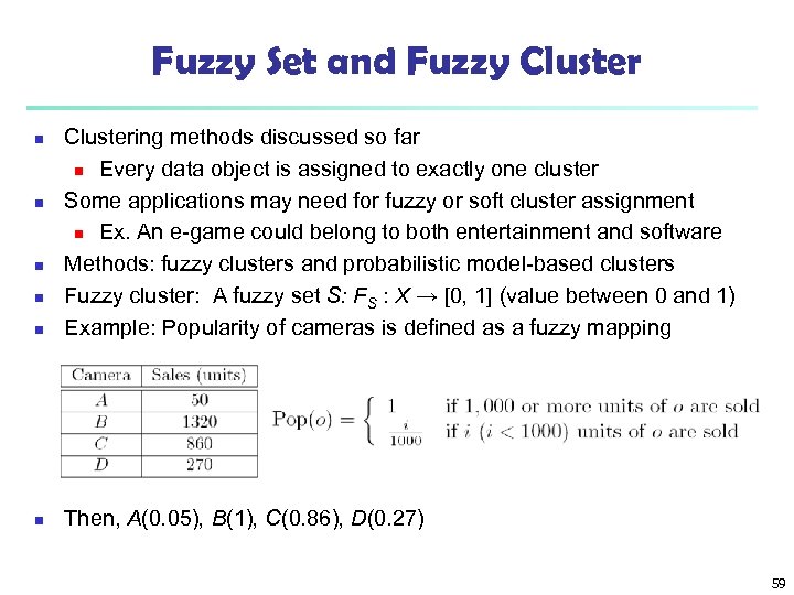
Fuzzy Set and Fuzzy Cluster n Clustering methods discussed so far n Every data object is assigned to exactly one cluster Some applications may need for fuzzy or soft cluster assignment n Ex. An e-game could belong to both entertainment and software Methods: fuzzy clusters and probabilistic model-based clusters Fuzzy cluster: A fuzzy set S: FS : X → [0, 1] (value between 0 and 1) Example: Popularity of cameras is defined as a fuzzy mapping n Then, A(0. 05), B(1), C(0. 86), D(0. 27) n n 59
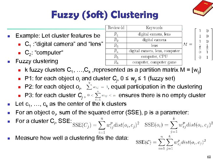
Fuzzy (Soft) Clustering n Example: Let cluster features be n C 1 : “digital camera” and “lens” n C 2: “computer“ Fuzzy clustering n k fuzzy clusters C 1, …, Ck , represented as a partition matrix M = [wij] n P 1: for each object oi and cluster Cj, 0 ≤ wij ≤ 1 (fuzzy set) n P 2: for each object oi, , equal participation in the clustering n P 3: for each cluster Cj , ensures there is no empty cluster Let c 1, …, ck as the center of the k clusters For an object oi, sum of the squared error (SSE), p is a parameter: For a cluster Ci, SSE: n Measure how well a clustering fits the data: n n 60
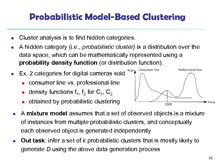
Probabilistic Model-Based Clustering n n n Cluster analysis is to find hidden categories. A hidden category (i. e. , probabilistic cluster) is a distribution over the data space, which can be mathematically represented using a probability density function (or distribution function). Ex. 2 categories for digital cameras sold n n n density functions f 1, f 2 for C 1, C 2 n n consumer line vs. professional line obtained by probabilistic clustering A mixture model assumes that a set of observed objects is a mixture of instances from multiple probabilistic clusters, and conceptually each observed object is generated independently Out task: infer a set of k probabilistic clusters that is mostly likely to generate D using the above data generation process 61
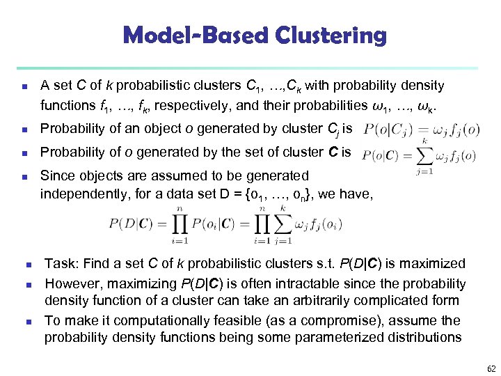
Model-Based Clustering n A set C of k probabilistic clusters C 1, …, Ck with probability density functions f 1, …, fk, respectively, and their probabilities ω1, …, ωk. n Probability of an object o generated by cluster Cj is n Probability of o generated by the set of cluster C is n n Since objects are assumed to be generated independently, for a data set D = {o 1, …, on}, we have, Task: Find a set C of k probabilistic clusters s. t. P(D|C) is maximized However, maximizing P(D|C) is often intractable since the probability density function of a cluster can take an arbitrarily complicated form To make it computationally feasible (as a compromise), assume the probability density functions being some parameterized distributions 62
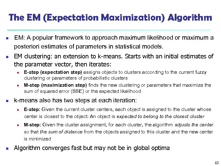
The EM (Expectation Maximization) Algorithm n n EM: A popular framework to approach maximum likelihood or maximum a posteriori estimates of parameters in statistical models. EM clustering: an extension to k-means. Starts with an initial estimates of the parameter vector, then iterates: n n n k-means also has two steps at each iteration: n n n E-step (expectation step) assigns objects to clusters according to the current fuzzy clustering or parameters of probabilistic clusters M-step (maximization step) finds the new clustering or parameters that maximize the sum of squared error (SSE) or the expected likelihood E-step: Given the current cluster centers, each object is assigned to the cluster whose center is closest to the object: An object is expected to belong to the closest cluster M-step: Given the cluster assignment, for each cluster, the algorithm adjusts the center so that the sum of distance from the objects assigned to this cluster and the new center is minimized Algorithm converges fast but may not be in global optima 63
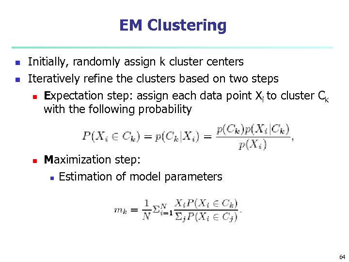
EM Clustering n n Initially, randomly assign k cluster centers Iteratively refine the clusters based on two steps n Expectation step: assign each data point X i to cluster Ck with the following probability n Maximization step: n Estimation of model parameters 64
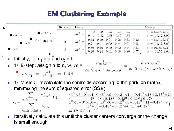
EM Clustering Example n n Initially, let c 1 = a and c 2 = b 1 st E-step: assign o to c 1, w. wt = n n n 1 st M-step: recalculate the centroids according to the partition matrix, minimizing the sum of squared error (SSE) Iteratively calculate this until the cluster centers converge or the change is small enough 65
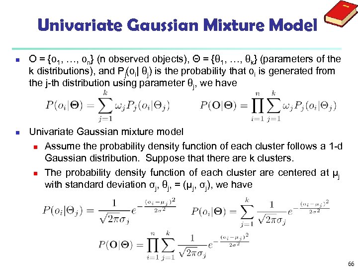
Univariate Gaussian Mixture Model n n O = {o 1, …, on} (n observed objects), Θ = {θ 1, …, θk} (parameters of the k distributions), and Pj(oi| θj) is the probability that oi is generated from the j-th distribution using parameter θj, we have Univariate Gaussian mixture model n Assume the probability density function of each cluster follows a 1 -d Gaussian distribution. Suppose that there are k clusters. n The probability density function of each cluster are centered at μj with standard deviation σj, θj, = (μj, σj), we have 66
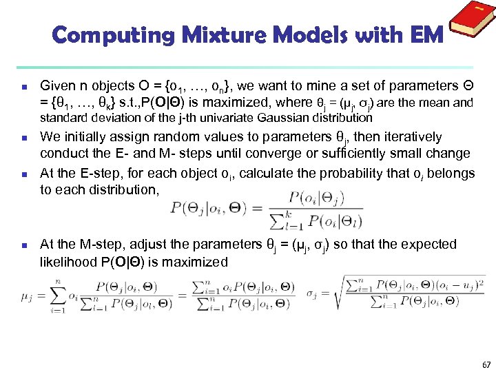
Computing Mixture Models with EM n Given n objects O = {o 1, …, on}, we want to mine a set of parameters Θ = {θ 1, …, θk} s. t. , P(O|Θ) is maximized, where θj = (μj, σj) are the mean and standard deviation of the j-th univariate Gaussian distribution n We initially assign random values to parameters θj, then iteratively conduct the E- and M- steps until converge or sufficiently small change At the E-step, for each object oi, calculate the probability that oi belongs to each distribution, At the M-step, adjust the parameters θj = (μj, σj) so that the expected likelihood P(O|Θ) is maximized 67
Strengths and Weaknesses of Mixture Models n Strength n n Mixture models are more general than partitioning and fuzzy clustering Clusters can be characterized by a small number of parameters The results may satisfy the statistical assumptions of the generative models Weakness n n Converge to local optimal (overcome: run multi-times w. random initialization) Computationally expensive if the number of distributions is large, or the data set contains very few observed data points n Need large data sets n Hard to estimate the number of clusters 68
Chapter 11. Cluster Analysis: Advanced Methods n Probability Model-Based Clustering n Clustering High-Dimensional Data n Clustering Graphs and Network Data n Clustering with Constraints 69
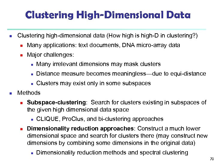
Clustering High-Dimensional Data n Clustering high-dimensional data (How high is high-D in clustering? ) n Many applications: text documents, DNA micro-array data n Major challenges: n n Distance measure becomes meaningless—due to equi-distance n n Many irrelevant dimensions may mask clusters Clusters may exist only in some subspaces Methods n Subspace-clustering: Search for clusters existing in subspaces of the given high dimensional data space n n CLIQUE, Pro. Clus, and bi-clustering approaches Dimensionality reduction approaches: Construct a much lower dimensional space and search for clusters there (may construct new dimensions by combining some dimensions in the original data) n Dimensionality reduction methods and spectral clustering 70
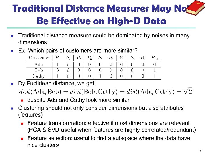
Traditional Distance Measures May Not Be Effective on High-D Data n Traditional distance measure could be dominated by noises in many dimensions Ex. Which pairs of customers are more similar? n By Euclidean distance, we get, n despite Ada and Cathy look more similar Clustering should not only consider dimensions but also attributes (features) n Feature transformation: effective if most dimensions are relevant (PCA & SVD useful when features are highly correlated/redundant) n Feature selection: useful to find a subspace where the data have nice clusters n n 71
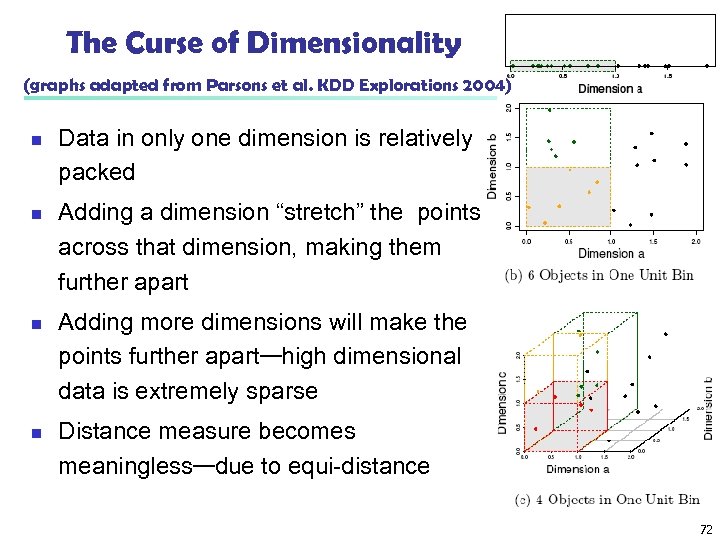
The Curse of Dimensionality (graphs adapted from Parsons et al. KDD Explorations 2004) n n Data in only one dimension is relatively packed Adding a dimension “stretch” the points across that dimension, making them further apart Adding more dimensions will make the points further apart—high dimensional data is extremely sparse Distance measure becomes meaningless—due to equi-distance 72
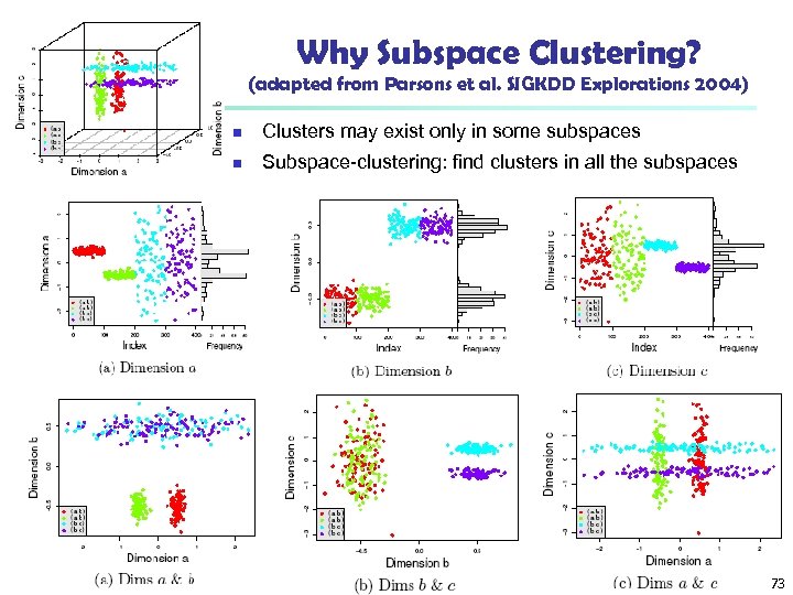
Why Subspace Clustering? (adapted from Parsons et al. SIGKDD Explorations 2004) n Clusters may exist only in some subspaces n Subspace-clustering: find clusters in all the subspaces 73
Subspace Clustering Methods n Subspace search methods: Search various subspaces to find clusters n n n Bottom-up approaches Top-down approaches Correlation-based clustering methods n n E. g. , PCA based approaches Bi-clustering methods n Optimization-based methods n Enumeration methods 74
Subspace Clustering Method (I): Subspace Search Methods n Search various subspaces to find clusters n Bottom-up approaches n n Start from low-D subspaces and search higher-D subspaces only when there may be clusters in such subspaces Various pruning techniques to reduce the number of higher-D subspaces to be searched Ex. CLIQUE (Agrawal et al. 1998) Top-down approaches n n n Start from full space and search smaller subspaces recursively Effective only if the locality assumption holds: restricts that the subspace of a cluster can be determined by the local neighborhood Ex. PROCLUS (Aggarwal et al. 1999): a k-medoid-like method 75
CLIQUE (Sub. Space Clustering with Aprori Pruning) n n n Agrawal, Gehrke, Gunopulos, Raghavan (SIGMOD’ 98) Automatically identifying subspaces of a high dimensional data space that allow better clustering than original space CLIQUE can be considered as both density-based and grid-based n n It partitions each dimension into the same number of equal length interval It partitions an m-dimensional data space into non-overlapping rectangular units A unit is dense if the fraction of total data points contained in the unit exceeds the input model parameter A cluster is a maximal set of connected dense units within a subspace 76
CLIQUE: The Major Steps n n n Partition the data space and find the number of points that lie inside each cell of the partition. Identify the subspaces that contain clusters using the Apriori principle Identify clusters n n n Determine dense units in all subspaces of interests Determine connected dense units in all subspaces of interests. Generate minimal description for the clusters n Determine maximal regions that cover a cluster of connected dense units for each cluster n Determination of minimal cover for each cluster 77
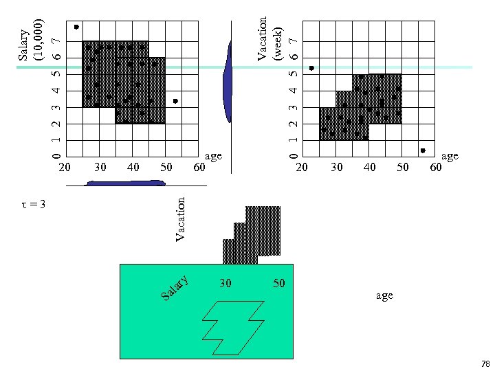
30 40 =3 Vacation 20 50 S Salary (10, 000) 0 1 2 3 4 5 6 7 a al ry 30 Vacation (week) 0 1 2 3 4 5 6 7 age 60 20 50 30 40 50 age 60 age 78
Strength and Weakness of CLIQUE n Strength n n automatically finds subspaces of the highest dimensionality such that high density clusters exist in those subspaces n insensitive to the order of records in input and does not presume some canonical data distribution n scales linearly with the size of input and has good scalability as the number of dimensions in the data increases Weakness n The accuracy of the clustering result may be degraded at the expense of simplicity of the method 79
Bi-Clustering Methods n n Real-world data is noisy: Try to find approximate bi-clusters Methods: Optimization-based methods vs. enumeration methods Optimization-based methods n Try to find a submatrix at a time that achieves the best significance as a bi-cluster n Due to the cost in computation, greedy search is employed to find local optimal bi-clusters n Ex. δ-Cluster Algorithm (Cheng and Church, ISMB’ 2000) Enumeration methods n Use a tolerance threshold to specify the degree of noise allowed in the bi-clusters to be mined n Then try to enumerate all submatrices as bi-clusters that satisfy the requirements n Ex. δ-p. Cluster Algorithm (H. Wang et al. ’ SIGMOD’ 2002, Ma. Ple: Pei et al. , ICDM’ 2003) 80
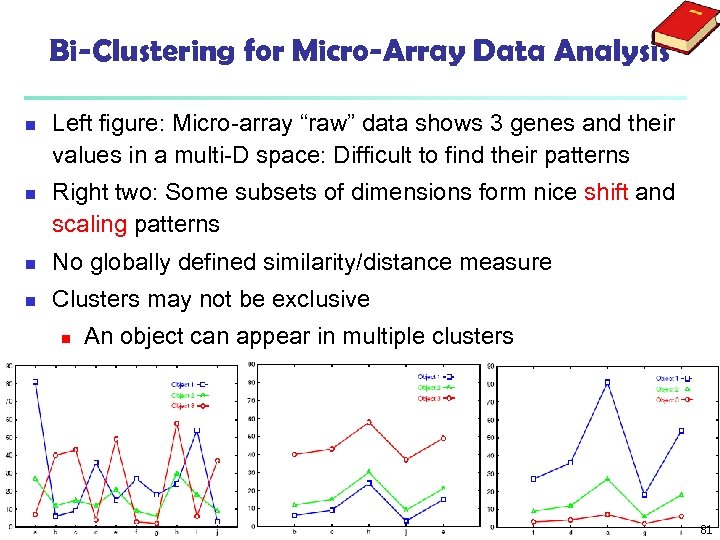
Bi-Clustering for Micro-Array Data Analysis n n Left figure: Micro-array “raw” data shows 3 genes and their values in a multi-D space: Difficult to find their patterns Right two: Some subsets of dimensions form nice shift and scaling patterns n No globally defined similarity/distance measure n Clusters may not be exclusive n An object can appear in multiple clusters 81
Chapter 11. Cluster Analysis: Advanced Methods n Probability Model-Based Clustering n Clustering High-Dimensional Data n Clustering Graphs and Network Data n Clustering with Constraints 82
Clustering Graphs and Network Data n n n Applications n Bi-partite graphs, e. g. , customers and products, authors and conferences n Web search engines, e. g. , click through graphs and Web graphs n Social networks, friendship/coauthor graphs Similarity measures n Geodesic distances n Distance based on random walk (Sim. Rank) Graph clustering methods n Minimum cuts: Fast. Modularity (Clauset, Newman & Moore, 2004) n Density-based clustering: SCAN (Xu et al. , KDD’ 2007) 83
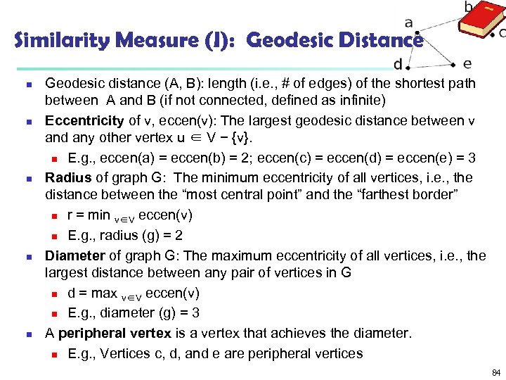
Similarity Measure (I): Geodesic Distance n n n Geodesic distance (A, B): length (i. e. , # of edges) of the shortest path between A and B (if not connected, defined as infinite) Eccentricity of v, eccen(v): The largest geodesic distance between v and any other vertex u ∈ V − {v}. n E. g. , eccen(a) = eccen(b) = 2; eccen(c) = eccen(d) = eccen(e) = 3 Radius of graph G: The minimum eccentricity of all vertices, i. e. , the distance between the “most central point” and the “farthest border” n r = min v∈V eccen(v) n E. g. , radius (g) = 2 Diameter of graph G: The maximum eccentricity of all vertices, i. e. , the largest distance between any pair of vertices in G n d = max v∈V eccen(v) n E. g. , diameter (g) = 3 A peripheral vertex is a vertex that achieves the diameter. n E. g. , Vertices c, d, and e are peripheral vertices 84
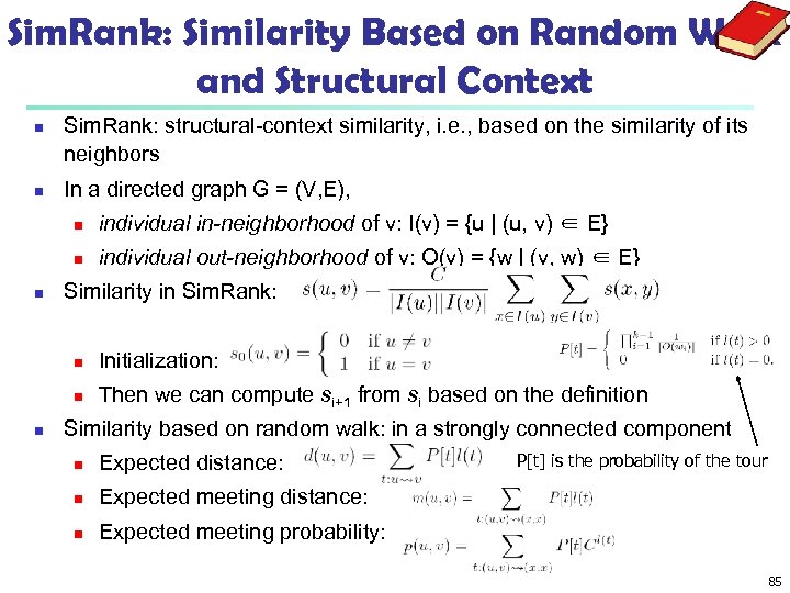
Sim. Rank: Similarity Based on Random Walk and Structural Context n n Sim. Rank: structural-context similarity, i. e. , based on the similarity of its neighbors In a directed graph G = (V, E), n n n individual in-neighborhood of v: I(v) = {u | (u, v) ∈ E} individual out-neighborhood of v: O(v) = {w | (v, w) ∈ E} Similarity in Sim. Rank: n n n Initialization: Then we can compute si+1 from si based on the definition Similarity based on random walk: in a strongly connected component n Expected distance: n Expected meeting distance: n P[t] is the probability of the tour Expected meeting probability: 85
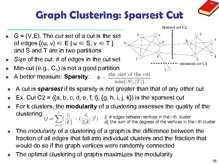
Graph Clustering: Sparsest Cut n n n n G = (V, E). The cut set of a cut is the set of edges {(u, v) ∈ E | u ∈ S, v ∈ T } and S and T are in two partitions Size of the cut: # of edges in the cut set Min-cut (e. g. , C 1) is not a good partition A better measure: Sparsity: A cut is sparsest if its sparsity is not greater than that of any other cut Ex. Cut C 2 = ({a, b, c, d, e, f, l}, {g, h, i, j, k}) is the sparsest cut For k clusters, the modularity of a clustering assesses the quality of the clustering: l : # edges between vertices in the i-th cluster i di: the sum of the degrees of the vertices in the i-th cluster n n The modularity of a clustering of a graph is the difference between the fraction of all edges that fall into individual clusters and the fraction that would do so if the graph vertices were randomly connected The optimal clustering of graphs maximizes the modularity 86
Graph Clustering: Challenges of Finding Good Cuts n n High computational cost n Many graph cut problems are computationally expensive n The sparsest cut problem is NP-hard n Need to tradeoff between efficiency/scalability and quality Sophisticated graphs n May involve weights and/or cycles. High dimensionality n A graph can have many vertices. In a similarity matrix, a vertex is represented as a vector (a row in the matrix) whose dimensionality is the number of vertices in the graph Sparsity n A large graph is often sparse, meaning each vertex on average connects to only a small number of other vertices n A similarity matrix from a large sparse graph can also be sparse 87
Two Approaches for Graph Clustering n Two approaches for clustering graph data n n n Use generic clustering methods for high-dimensional data Designed specifically for clustering graphs Using clustering methods for high-dimensional data n n Extract a similarity matrix from a graph using a similarity measure A generic clustering method can then be applied on the similarity matrix to discover clusters Ex. Spectral clustering: approximate optimal graph cut solutions Methods specific to graphs n Search the graph to find well-connected components as clusters n Ex. SCAN (Structural Clustering Algorithm for Networks) n X. Xu, N. Yuruk, Z. Feng, and T. A. J. Schweiger, “SCAN: A Structural Clustering Algorithm for Networks”, KDD'07 88
Chapter 11. Cluster Analysis: Advanced Methods n Probability Model-Based Clustering n Clustering High-Dimensional Data n Clustering Graphs and Network Data n Clustering with Constraints 89
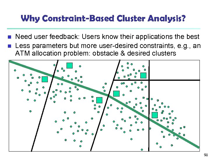
Why Constraint-Based Cluster Analysis? Need user feedback: Users know their applications the best n Less parameters but more user-desired constraints, e. g. , an ATM allocation problem: obstacle & desired clusters n 90
Categorization of Constraints n Constraints on instances: specifies how a pair or a set of instances should be grouped in the cluster analysis n Must-link vs. cannot link constraints n n Constraints can be defined using variables, e. g. , n n E. g. , specify the min # of objects in a cluster, the max diameter of a cluster, the shape of a cluster (e. g. , a convex), # of clusters (e. g. , k) Constraints on similarity measurements: specifies a requirement that the similarity calculation must respect n n cannot-link(x, y) if dist(x, y) > d Constraints on clusters: specifies a requirement on the clusters n n must-link(x, y): x and y should be grouped into one cluster E. g. , driving on roads, obstacles (e. g. , rivers, lakes) Issues: Hard vs. soft constraints; conflicting or redundant constraints 91
Constraint-Based Clustering Methods (I): Handling Hard Constraints n n Handling hard constraints: Strictly respect the constraints in cluster assignments Example: The COP-k-means algorithm n Generate super-instances for must-link constraints n Compute the transitive closure of the must-link constraints n To represent such a subset, replace all those objects in the subset by the mean. n The super-instance also carries a weight, which is the number of objects it represents n Conduct modified k-means clustering to respect cannot-link constraints n Modify the center-assignment process in k-means to a nearest feasible center assignment n An object is assigned to the nearest center so that the assignment respects all cannot-link constraints 92
Constraint-Based Clustering Methods (II): Handling Soft Constraints n n Treated as an optimization problem: When a clustering violates a soft constraint, a penalty is imposed on the clustering Overall objective: Optimizing the clustering quality, and minimizing the constraint violation penalty Ex. CVQE (Constrained Vector Quantization Error) algorithm: Conduct k-means clustering while enforcing constraint violation penalties Objective function: Sum of distance used in k-means, adjusted by the constraint violation penalties n Penalty of a must-link violation n If objects x and y must-be-linked but they are assigned to two different centers, c 1 and c 2, dist(c 1, c 2) is added to the objective function as the penalty n Penalty of a cannot-link violation n If objects x and y cannot-be-linked but they are assigned to a common center c, dist(c, c′), between c and c′ is added to the objective function as the penalty, where c′ is the closest cluster to c that can accommodate x or y 93
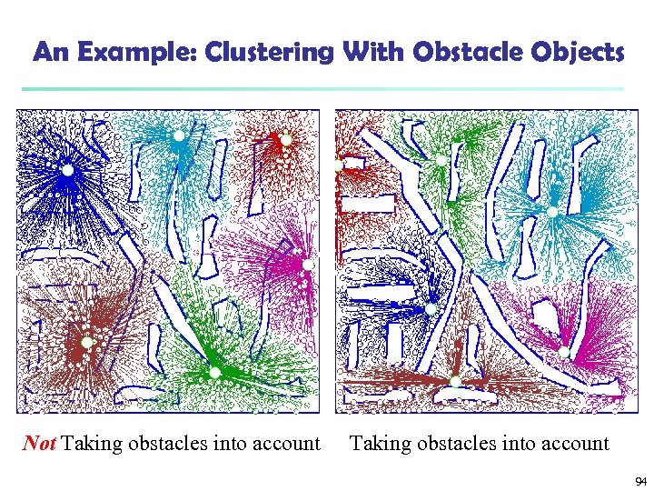
An Example: Clustering With Obstacle Objects Not Taking obstacles into account 94
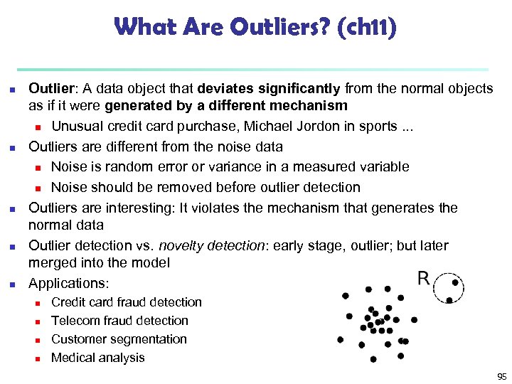
What Are Outliers? (ch 11) n n n Outlier: A data object that deviates significantly from the normal objects as if it were generated by a different mechanism n Unusual credit card purchase, Michael Jordon in sports. . . Outliers are different from the noise data n Noise is random error or variance in a measured variable n Noise should be removed before outlier detection Outliers are interesting: It violates the mechanism that generates the normal data Outlier detection vs. novelty detection: early stage, outlier; but later merged into the model Applications: n n Credit card fraud detection Telecom fraud detection Customer segmentation Medical analysis 95
9d9b06a1cec5d47a68c7f8f6361f990c.ppt