83a71dc0e6ac9c4156d2e7b7b1462e0e.ppt
- Количество слайдов: 44

Chapter 10 Association between Random Variables Copyright © 2011 Pearson Education, Inc.
10. 1 Portfolios and Random Variables How should money be allocated among several stocks that form a portfolio? § Need to manipulate several random variables at once to understand portfolios § Since stocks tend to rise and fall together, random variables for these events must capture dependence 3 of 44 Copyright © 2011 Pearson Education, Inc.
10. 1 Portfolios and Random Variables Two Random Variables § Suppose a day trader can buy stock in two companies, IBM and Microsoft, at $100 per share § X denotes the change in value of IBM § Y denotes the change in value of Microsoft 4 of 44 Copyright © 2011 Pearson Education, Inc.
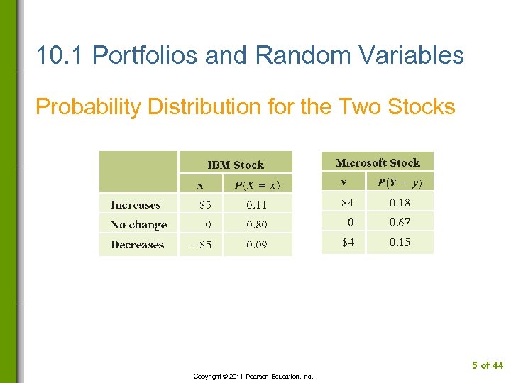
10. 1 Portfolios and Random Variables Probability Distribution for the Two Stocks 5 of 44 Copyright © 2011 Pearson Education, Inc.
10. 1 Portfolios and Random Variables Comparisons and the Sharpe Ratio The day trader can invest $200 in § § § Two shares of IBM; Two shares of Microsoft; or One share of each 6 of 44 Copyright © 2011 Pearson Education, Inc.
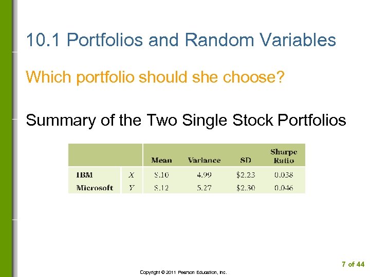
10. 1 Portfolios and Random Variables Which portfolio should she choose? Summary of the Two Single Stock Portfolios 7 of 44 Copyright © 2011 Pearson Education, Inc.
10. 2 Joint Probability Distribution Find Sharpe Ratio for Two Stock Portfolio § § Combines two different random variables (X and Y) that are not independent Need joint probability distribution that gives probabilities for events of the form (X = x and Y = y) 8 of 44 Copyright © 2011 Pearson Education, Inc.
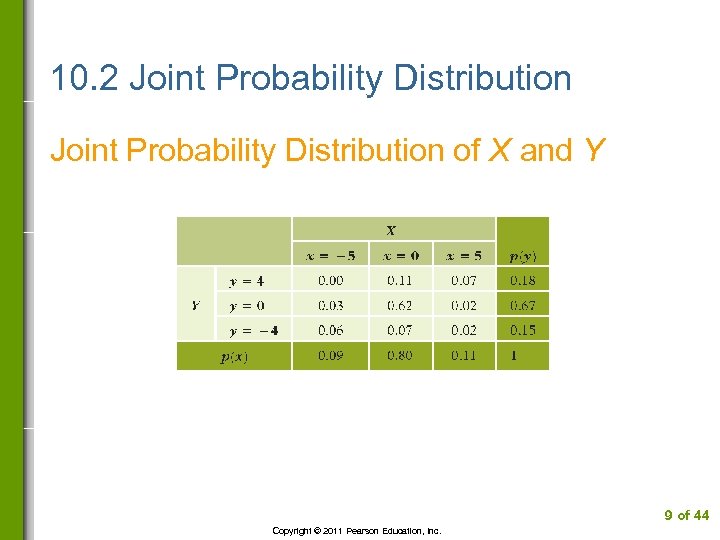
10. 2 Joint Probability Distribution of X and Y 9 of 44 Copyright © 2011 Pearson Education, Inc.
10. 2 Joint Probability Distribution Independent Random Variables Two random variables are independent if (and only if) the joint probability distribution is the product of the marginal distributions. p(x, y) = p(x) p(y) for all x, y 10 of 44 Copyright © 2011 Pearson Education, Inc.
10. 2 Joint Probability Distribution Multiplication Rule The expected value of a product of independent random variables is the product of their expected values. E(XY) = E(X)E(Y) 11 of 44 Copyright © 2011 Pearson Education, Inc.
4 M Example 10. 1: EXCHANGE RATES Motivation A firm’s sales in Europe average 10 million € each month. The current exchange rate is 1. 40$/€ but it fluctuates. What should this firm expect for the dollar value of European sales next month? 12 of 44 Copyright © 2011 Pearson Education, Inc.
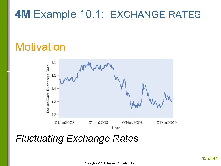
4 M Example 10. 1: EXCHANGE RATES Motivation Fluctuating Exchange Rates 13 of 44 Copyright © 2011 Pearson Education, Inc.
4 M Example 10. 1: EXCHANGE RATES Method Identify three random variables: S = sales next month in €; R = exchange rate next month; and D = value of sales in $. These are related by D = S R. Find E(D). 14 of 44 Copyright © 2011 Pearson Education, Inc.
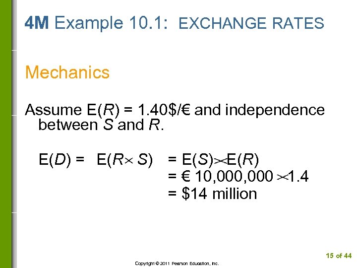
4 M Example 10. 1: EXCHANGE RATES Mechanics Assume E(R) = 1. 40$/€ and independence between S and R. E(D) = E(R S) = E(S) E(R) = € 10, 000 1. 4 = $14 million 15 of 44 Copyright © 2011 Pearson Education, Inc.
4 M Example 10. 1: EXCHANGE RATES Message European sales for next month convert to $14 million, on average. We assume that sales next month are, on average, the same as in the past for this firm and that sales and exchange rate are independent. 16 of 44 Copyright © 2011 Pearson Education, Inc.
10. 2 Joint Probability Distribution Dependent Random Variables § § Joint probability table shows changes in values of IBM and Microsoft (X and Y) are dependent The dependence between them is positive 17 of 44 Copyright © 2011 Pearson Education, Inc.
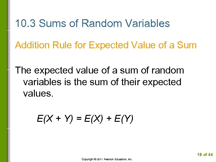
10. 3 Sums of Random Variables Addition Rule for Expected Value of a Sum The expected value of a sum of random variables is the sum of their expected values. E(X + Y) = E(X) + E(Y) 18 of 44 Copyright © 2011 Pearson Education, Inc.
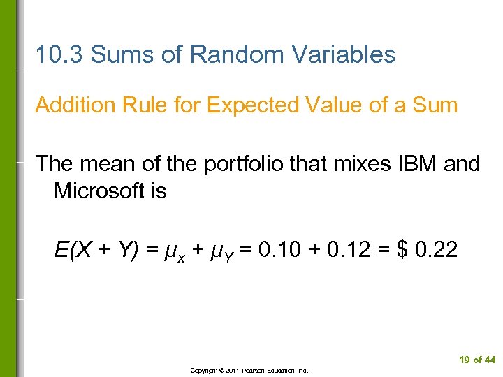
10. 3 Sums of Random Variables Addition Rule for Expected Value of a Sum The mean of the portfolio that mixes IBM and Microsoft is E(X + Y) = µx + µY = 0. 10 + 0. 12 = $ 0. 22 19 of 44 Copyright © 2011 Pearson Education, Inc.
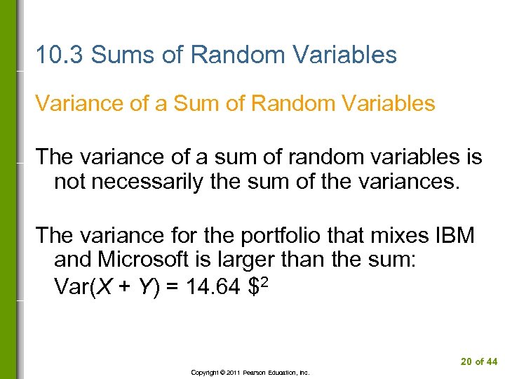
10. 3 Sums of Random Variables Variance of a Sum of Random Variables The variance of a sum of random variables is not necessarily the sum of the variances. The variance for the portfolio that mixes IBM and Microsoft is larger than the sum: Var(X + Y) = 14. 64 $2 20 of 44 Copyright © 2011 Pearson Education, Inc.
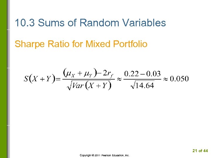
10. 3 Sums of Random Variables Sharpe Ratio for Mixed Portfolio 21 of 44 Copyright © 2011 Pearson Education, Inc.
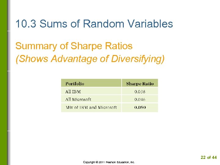
10. 3 Sums of Random Variables Summary of Sharpe Ratios (Shows Advantage of Diversifying) 22 of 44 Copyright © 2011 Pearson Education, Inc.
10. 4 Dependence Between Random Variables Covariance The covariance between random variables is the expected value of the product of deviations from the means. Cov(X, Y) = E((X - µX) (Y - µY)) 23 of 44 Copyright © 2011 Pearson Education, Inc.
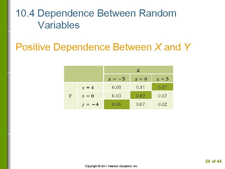
10. 4 Dependence Between Random Variables Positive Dependence Between X and Y 24 of 44 Copyright © 2011 Pearson Education, Inc.
10. 4 Dependence Between Random Variables Covariance and Sums The variance of the sum of two random variables is the sum of their variances plus twice their covariance. Var(X + Y) = Var(X) + Var(Y) + 2 Cov(X, Y) 25 of 44 Copyright © 2011 Pearson Education, Inc.
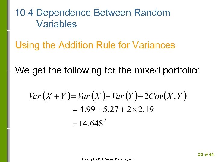
10. 4 Dependence Between Random Variables Using the Addition Rule for Variances We get the following for the mixed portfolio: 26 of 44 Copyright © 2011 Pearson Education, Inc.
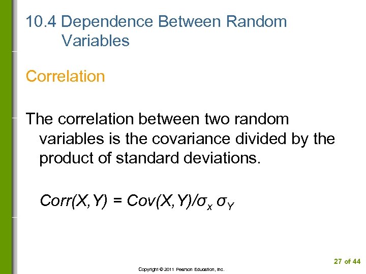
10. 4 Dependence Between Random Variables Correlation The correlation between two random variables is the covariance divided by the product of standard deviations. Corr(X, Y) = Cov(X, Y)/σx σY 27 of 44 Copyright © 2011 Pearson Education, Inc.
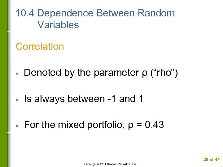
10. 4 Dependence Between Random Variables Correlation § Denoted by the parameter ρ (“rho”) § Is always between -1 and 1 § For the mixed portfolio, ρ = 0. 43 28 of 44 Copyright © 2011 Pearson Education, Inc.
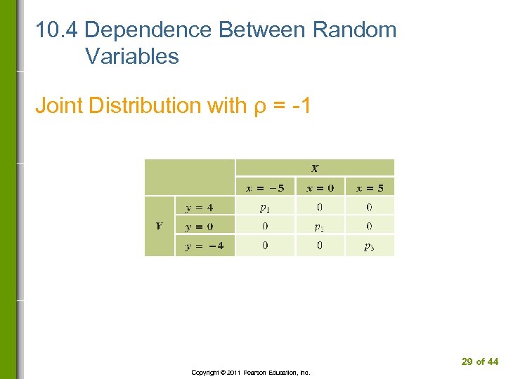
10. 4 Dependence Between Random Variables Joint Distribution with ρ = -1 29 of 44 Copyright © 2011 Pearson Education, Inc.

10. 4 Dependence Between Random Variables Joint Distribution with ρ = 1 30 of 44 Copyright © 2011 Pearson Education, Inc.
10. 4 Dependence Between Random Variables Covariance, Correlation and Independence § § A correlation of zero does not necessarily imply independence Independence does imply that the covariance and correlation are zero 31 of 44 Copyright © 2011 Pearson Education, Inc.
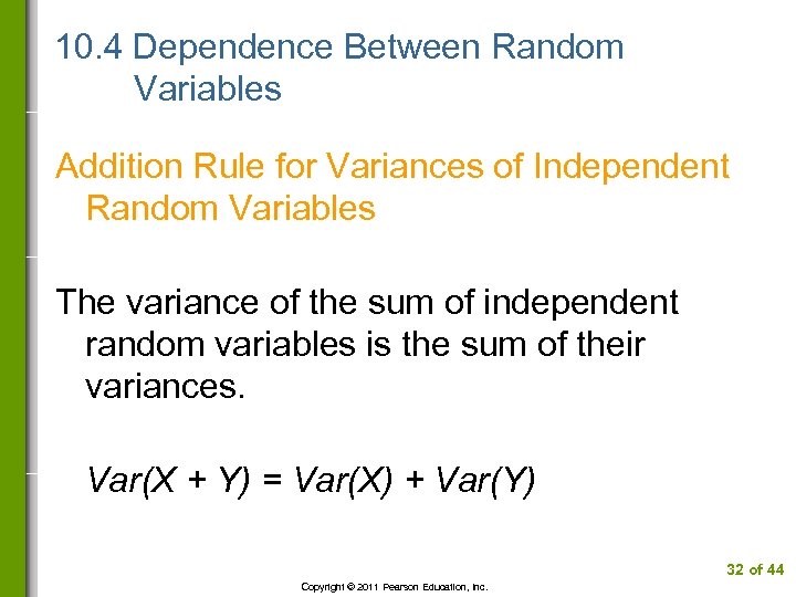
10. 4 Dependence Between Random Variables Addition Rule for Variances of Independent Random Variables The variance of the sum of independent random variables is the sum of their variances. Var(X + Y) = Var(X) + Var(Y) 32 of 44 Copyright © 2011 Pearson Education, Inc.
10. 5 IID Random Variables Definition § § Random variables that are independent of each other and share a common probability distribution are said to be independent and identically distributed. iid for short 33 of 44 Copyright © 2011 Pearson Education, Inc.
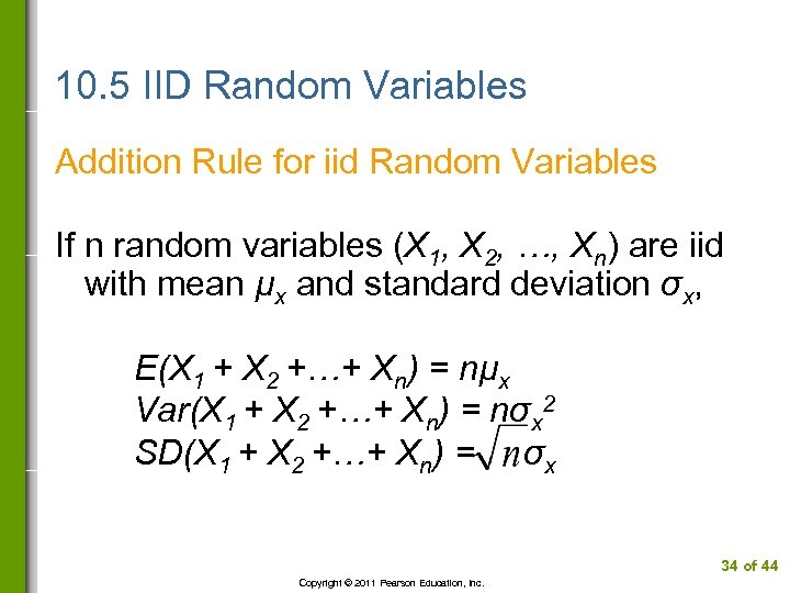
10. 5 IID Random Variables Addition Rule for iid Random Variables If n random variables (X 1, X 2, …, Xn) are iid with mean µx and standard deviation σx, E(X 1 + X 2 +…+ Xn) = nµx Var(X 1 + X 2 +…+ Xn) = nσx 2 SD(X 1 + X 2 +…+ Xn) = σx 34 of 44 Copyright © 2011 Pearson Education, Inc.
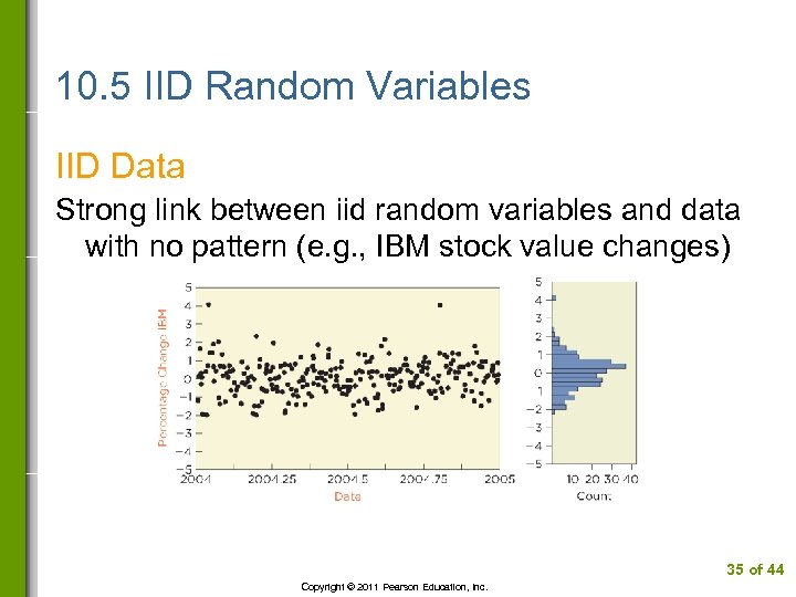
10. 5 IID Random Variables IID Data Strong link between iid random variables and data with no pattern (e. g. , IBM stock value changes) 35 of 44 Copyright © 2011 Pearson Education, Inc.
10. 6 Weighted Sums Addition Rule for Weighted Sums The expected value of a weighted sum of random variables is the weighted sum of the expected values. E(a. X + b. Y + c) = a. E(X) + b. E(Y) + c 36 of 44 Copyright © 2011 Pearson Education, Inc.
10. 6 Weighted Sums Addition Rule for Weighted Sums The variance of a weighted sum of random variables is Var(a. X + b. Y + c) = a 2 Var(X) + b 2 Var(Y) + 2 ab. Cov(X, Y) 37 of 44 Copyright © 2011 Pearson Education, Inc.
4 M Example 10. 2: CONSTRUCTION ESTIMATES Motivation Adding an addition to a home typically takes two carpenters working 240 hours with a standard deviation of 40 hours. Electrical work takes an average of 12 hours with standard deviation 4 hours. Carpenters charge $45/hour and electricians charge $80/hour. The amount of both types of labor could vary with ρ =0. 5. What is the total expected labor cost? 38 of 44 Copyright © 2011 Pearson Education, Inc.
4 M Example 10. 2: CONSTRUCTION ESTIMATES Method Identify three random variables: X = number of carpentry hours; Y = number of electrician hours; and T = total costs ($). These are related by T = 45 X + 80 Y. 39 of 44 Copyright © 2011 Pearson Education, Inc.
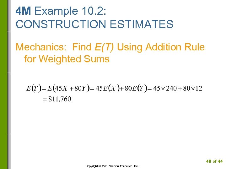
4 M Example 10. 2: CONSTRUCTION ESTIMATES Mechanics: Find E(T) Using Addition Rule for Weighted Sums 40 of 44 Copyright © 2011 Pearson Education, Inc.
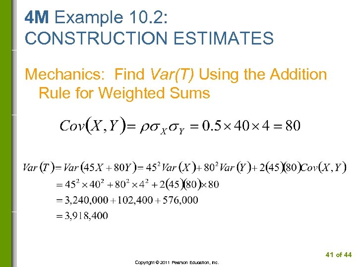
4 M Example 10. 2: CONSTRUCTION ESTIMATES Mechanics: Find Var(T) Using the Addition Rule for Weighted Sums 41 of 44 Copyright © 2011 Pearson Education, Inc.
4 M Example 10. 2: CONSTRUCTION ESTIMATES Message The expected total cost for labor is around $12, 000 with a standard deviation of about $2, 000. 42 of 44 Copyright © 2011 Pearson Education, Inc.
Best Practices § Consider the possibility of dependence. § Only add variances for random variables that are uncorrelated. § Use several random variables to capture different features of a problem. § Use new symbols for each random variable. 43 of 44 Copyright © 2011 Pearson Education, Inc.
Pitfalls § Do not think that uncorrelated random variables are independent. § Don’t forget the covariance when finding the variance of a sum. § Never add standard deviations of random variables. § Don’t mistake Var(X – Y) for Var(X) – Var(Y). 44 of 44 Copyright © 2011 Pearson Education, Inc.
83a71dc0e6ac9c4156d2e7b7b1462e0e.ppt